Introduction
AMRgen is a comprehensive R package designed to
integrate antimicrobial resistance genotype and phenotype data. It
provides tools to:
Import AMR genotype data (e.g. from AMRFinderPlus, hAMRonization)
Import AST phenotype data (e.g. public data from NCBI or EBI, or your own data in formats like Vitek or WHOnet)
Conduct genotype-phenotype analyses to explore the impact of genotypic markers on phenotype, including via logistic regression, solo marker analysis, and upset plots
Fetch MIC or disk zone reference distributions from EUCAST
This vignette walks through a basic workflow using example datasets
included in the AMRgen package, and explains how to wrangle
your own data files into the right formats to use the same workflow.
Start by loading the package:
library(AMRgen)
library(dplyr)
#>
#> Attaching package: 'dplyr'
#> The following objects are masked from 'package:stats':
#>
#>     filter, lag
#> The following objects are masked from 'package:base':
#>
#>     intersect, setdiff, setequal, union
1. Genotype table
1a. Importing genotype data to AMRgen’s standard table format
The import_amrfp() function lets you load genotype data
from AMRFinderPlus output files, and process it to generate an object
with the key columns needed to work with the AMRgen
package.
# Example AMRFinderPlus genotyping output (from AllTheBacteria project)
ecoli_geno_raw
#> # A tibble: 45,228 × 28
#>    Name      `Protein identifier` `Contig id`  Start   Stop Strand `Gene symbol`
#>    <chr>     <lgl>                <chr>        <dbl>  <dbl> <chr>  <chr>
#>  1 SAMN0317… NA                   SAMN031776…  74721  75851 -      blaEC
#>  2 SAMN0317… NA                   SAMN031776… 166214 169315 +      acrF
#>  3 SAMN0317… NA                   SAMN031776…  20678  22033 -      glpT_E448K
#>  4 SAMN0317… NA                   SAMN031776…    758   1969 -      floR
#>  5 SAMN0317… NA                   SAMN031776…   4440   5666 +      mdtM
#>  6 SAMN0317… NA                   SAMN031776…   3941   4798 +      blaTEM-1
#>  7 SAMN0317… NA                   SAMN031776…    142    954 +      sul2
#>  8 SAMN0317… NA                   SAMN031776…   1018   1818 +      aph(3'')-Ib
#>  9 SAMN0317… NA                   SAMN031776…   1821   2654 +      aph(6)-Id
#> 10 SAMN0317… NA                   SAMN031776…    788   1957 +      tet(A)
#> # ℹ 45,218 more rows
#> # ℹ 21 more variables: `Sequence name` <chr>, Scope <chr>,
#> #   `Element type` <chr>, `Element subtype` <chr>, Class <chr>, Subclass <chr>,
#> #   Method <chr>, `Target length` <dbl>, `Reference sequence length` <dbl>,
#> #   `% Coverage of reference sequence` <dbl>,
#> #   `% Identity to reference sequence` <dbl>, `Alignment length` <dbl>,
#> #   `Accession of closest sequence` <chr>, `Name of closest sequence` <chr>, …

# Load AMRFinderPlus output
ecoli_geno <- import_amrfp(
  input_table = ecoli_geno_raw, # (replace 'ecoli_geno_raw' with the filepath for any AMRFinderPlus output)
  sample_col = "Name",
  # you can optionally specify the below key column names if they differ in your dataframe to standard AMRFinderPlus outputs
  element_symbol_col = "Gene symbol", # or "Element symbol"
  element_type_col = "Element type", # or "Type"
  element_subtype_col = "Element subtype",
  method_col = "Method",
  node_col = "Hierarchy node",
  subclass_col = "Subclass",
  class_col = "Class"
)

# Check the format of the processed genotype table
head(ecoli_geno)
#> # A tibble: 6 × 37
#>   id           marker     gene  mutation drug drug_class  `variation type` node
#>   <chr>        <chr>      <chr> <chr>    <ab> <chr>       <chr>            <chr>
#> 1 SAMN03177615 blaEC      blaEC NA       NA   Beta-lacta… Gene presence d… blaEC
#> 2 SAMN03177615 acrF       acrF  NA       NA   Efflux      Gene presence d… acrF
#> 3 SAMN03177615 glpT_E448K glpT  Glu448L… FOS  Phosphonics Protein variant… glpT
#> 4 SAMN03177615 floR       floR  NA       CHL  Phenicols   Gene presence d… floR
#> 5 SAMN03177615 floR       floR  NA       FLR  Phenicols   Gene presence d… floR
#> 6 SAMN03177615 mdtM       mdtM  NA       NA   Efflux      Gene presence d… mdtM
#> # ℹ 29 more variables: marker.label <chr>, `Protein identifier` <lgl>,
#> #   `Contig id` <chr>, Start <dbl>, Stop <dbl>, Strand <chr>,
#> #   `Gene symbol` <chr>, `Sequence name` <chr>, Scope <chr>,
#> #   `Element type` <chr>, `Element subtype` <chr>, Class <chr>, Subclass <chr>,
#> #   Method <chr>, `Target length` <dbl>, `Reference sequence length` <dbl>,
#> #   `% Coverage of reference sequence` <dbl>,
#> #   `% Identity to reference sequence` <dbl>, `Alignment length` <dbl>, …
The genotype table has one row for each genetic marker detected in an input genome, i.e. one per strain/marker combination. This means your output table may end up with more columns than your input table, as markers conferring resistance to multiple drug classes will be expanded into several rows.
If your genotype data is not in AMRFinderPlus format, you can wrangle
other input data files into the necessary format. If only your column
names differ to standard AMRFinderPlus inputs, you can specify these
using element_symbol_col, element_type_col,
element_subtype_col, method_col,
node_col, subclass_col and
class_col.
The essential columns for a genotype table to work with downstream
AMRgen functions are:
id: character string giving the sample name, used to link to sample names in the phenotype file (this column can have a different name, in which case you’ll need to make sure it is the first column in the dataframe OR pass its name to the functions usinggeno_sample_col)marker: character string giving the name of the genetic marker detecteddrug_class: character string giving the antibiotic class associated with this marker
NOTE: You should consider whether you have genomes with no AMR
markers detected by genotyping, and how to make sure these are include
in your analyses. E.g. AMRFinderPlus will output one row per
genome/marker combination, but if you have a genome with no markers
detected, there will be no row at all for that genome in the
concatenated output file. If your species has core genes included in
AMRFinderPlus this probably won’t be a problem as you would expect some
calls for every genome (e.g. AMRFinderPlus will report blaSHV, oqxA,
oqxB, fosA in all Klebsiella pneumoniae genomes, so all input genomes
will appear in the concatenated output file). An easy solution is to run
a check to make sure that all genome names in your input dataset are
represented in the genotype table, and if any are missing add empty rows
for these using
e.g. tibble(Name=missing_samples) %>% bind_rows(genotype_table).
1b. Summarising a genotype table
You can summarise the content of a genotype table using the inbuilt
summarise_geno() function.
ecoli_geno_summary <- summarise_geno(ecoli_geno)

# Number of unique samples, markers, genes, drugs, classes, and variation types
ecoli_geno_summary$uniques
#> # A tibble: 6 × 2
#>   column         n_unique
#>   <chr>             <int>
#> 1 id                 5258
#> 2 marker              244
#> 3 drug                 35
#> 4 drug_class           26
#> 5 gene                196
#> 6 variation type        5

# Unique counts of samples, markers, genes, drugs, and classes - per variation type
ecoli_geno_summary$per_type
#> # A tibble: 5 × 6
#>   `variation type`                  id marker  drug drug_class  gene
#>   <chr>                          <int>  <int> <int>      <int> <int>
#> 1 Gene presence detected          5258    164    22         17   164
#> 2 Inactivating mutation detected   615     42    15         14    42
#> 3 Nucleotide variant detected       57      2     3          3     1
#> 4 Promoter variant detected         93      4     1          1     1
#> 5 Protein variant detected        4920     65    18         16    21
The summarise_geno() function also returns a list of
drugs and classes represented in the table, and the associated number of
unique markers, unique samples, and total hits for each drug/class.
Ordering by sample count, we see the most common class is efflux… there
are only 3 efflux-associated markers but there are 11,828 hits to these
across 5,258 samples (i.e. all samples have at least one). Next most
common are markers associated with beta-lactams… there are 22 different
markers with 6,379 hits across 4,989 of our 5,258 samples.
ecoli_geno_summary$drugs
#> # A tibble: 44 × 6
#>    drug drug_name                   drug_class       markers samples  hits
#>    <ab> <chr>                       <chr>              <int>   <int> <int>
#>  1 AMC  Amoxicillin/clavulanic acid Aminopenicillins       2      57    57
#>  2 AMK  Amikacin                    Aminoglycosides        6     176   180
#>  3 AMP  Ampicillin                  Aminopenicillins       6     749   749
#>  4 APR  Apramycin                   Aminoglycosides        1      98    98
#>  5 ATM  Aztreonam                   Monobactams            2      39    39
#>  6 AZM  Azithromycin                Macrolides             4     472   478
#>  7 BLM  Bleomycin                   Glycopeptides          2      40    40
#>  8 CHL  Chloramphenicol             Phenicols             15    1121  1181
#>  9 CLI  Clindamycin                 Lincosamides           1      26    26
#> 10 CLR  Clarithromycin              Macrolides             1       1     1
#> # ℹ 34 more rows

# Order by sample count per drug/class
ecoli_geno_summary$drugs %>% arrange(-samples)
#> # A tibble: 44 × 6
#>    drug drug_name       drug_class                markers samples  hits
#>    <ab> <chr>           <chr>                       <int>   <int> <int>
#>  1 NA   NA              Efflux                          3    5258 11828
#>  2 NA   NA              Beta-lactams                   22    4989  6379
#>  3 FOS  Fosfomycin      Phosphonics                     9    4861  6411
#>  4 COL  Colistin        Polymyxins                     11    3415  3436
#>  5 NA   NA              Tetracyclines                  13    2634  2929
#>  6 NA   NA              Quinolones                     45    1822  4497
#>  7 STR1 Streptomycin    Aminoglycosides                13    1669  3291
#>  8 SSS  Sulfonamide     Sulfonamides                    5    1500  1876
#>  9 CHL  Chloramphenicol Phenicols                      15    1121  1181
#> 10 NA   NA              Cephalosporins (3rd gen.)      32    1065  1285
#> # ℹ 34 more rows
Ordering by marker count, we see the classes with the most different markers associated are quinolones (45 unique markers detected across 1,822 unique samples), third generation cephalosporins (32 unique markers detected across 1,065 unique samples) and beta-lactams (22 unique markers detected across 4,989 unique samples).
ecoli_geno_summary$drugs %>% arrange(-markers)
#> # A tibble: 44 × 6
#>    drug drug_name       drug_class                markers samples  hits
#>    <ab> <chr>           <chr>                       <int>   <int> <int>
#>  1 NA   NA              Quinolones                     45    1822  4497
#>  2 NA   NA              Cephalosporins (3rd gen.)      32    1065  1285
#>  3 NA   NA              Beta-lactams                   22    4989  6379
#>  4 NA   NA              Trimethoprims                  16     824   877
#>  5 CHL  Chloramphenicol Phenicols                      15    1121  1181
#>  6 GEN  Gentamicin      Aminoglycosides                14     687   704
#>  7 STR1 Streptomycin    Aminoglycosides                13    1669  3291
#>  8 NA   NA              Carbapenems                    13      62    64
#>  9 NA   NA              Tetracyclines                  13    2634  2929
#> 10 COL  Colistin        Polymyxins                     11    3415  3436
#> # ℹ 34 more rows
The summarise_geno() function also returns a list of
markers represented in the table, annotated with the associated
drugs/classes and variation types. The column ‘n’ indicates the count of
hits detected per marker. Ordering by this column, we see the most
common markers are acrF, blaEC and glpT_E448K.
ecoli_geno_summary$markers %>% arrange(-n)
#> # A tibble: 349 × 6
#>    marker     drug drug_name  drug_class    `variation type`             n
#>    <chr>      <ab> <chr>      <chr>         <chr>                    <int>
#>  1 acrF       NA   NA         Efflux        Gene presence detected    5002
#>  2 blaEC      NA   NA         Beta-lactams  Gene presence detected    4749
#>  3 glpT_E448K FOS  Fosfomycin Phosphonics   Protein variant detected  4731
#>  4 mdtM       NA   NA         Efflux        Gene presence detected    3675
#>  5 emrD       NA   NA         Efflux        Gene presence detected    2914
#>  6 pmrB_E123D COL  Colistin   Polymyxins    Protein variant detected  1873
#>  7 pmrB_Y358N COL  Colistin   Polymyxins    Protein variant detected  1531
#>  8 blaTEM-1   NA   NA         Beta-lactams  Gene presence detected    1279
#>  9 uhpT_E350Q FOS  Fosfomycin Phosphonics   Protein variant detected  1145
#> 10 tet(A)     NA   NA         Tetracyclines Gene presence detected    1087
#> # ℹ 339 more rows
Filtering specifically for markers associated with quinolones, we can find out more about the 45 markers for this class that were found in the dataset. Summarising by variation type, we see there are 12 markers indicating detection of an acquired gene, 2 indicating inactivating mutaions, and 31 indicating protein mutations. Sorting by marker frequency, we can see the full list of 45 unique markers and that the most common is a protein variant in gyrA, gyrA_S83L. Filtering to “Gene presence detected” we can that the most common acquired gene was aac(6’)-Ib-cr5.
# Count the different types of variants found
ecoli_geno_summary$markers %>%
  filter(drug_class == "Quinolones") %>%
  count(`variation type`)
#> # A tibble: 3 × 2
#>   `variation type`                   n
#>   <chr>                          <int>
#> 1 Gene presence detected            12
#> 2 Inactivating mutation detected     2
#> 3 Protein variant detected          31

# Sort by marker frequency to see the most common markers
ecoli_geno_summary$markers %>%
  filter(drug_class == "Quinolones") %>%
  arrange(-n)
#> # A tibble: 45 × 6
#>    marker         drug drug_name drug_class `variation type`             n
#>    <chr>          <ab> <chr>     <chr>      <chr>                    <int>
#>  1 gyrA_S83L      NA   NA        Quinolones Protein variant detected   855
#>  2 marR_S3N       NA   NA        Quinolones Protein variant detected   726
#>  3 parC_S80I      NA   NA        Quinolones Protein variant detected   639
#>  4 gyrA_D87N      NA   NA        Quinolones Protein variant detected   622
#>  5 parE_I529L     NA   NA        Quinolones Protein variant detected   442
#>  6 parC_E84V      NA   NA        Quinolones Protein variant detected   294
#>  7 aac(6')-Ib-cr5 NA   NA        Quinolones Gene presence detected     153
#>  8 parE_D475E     NA   NA        Quinolones Protein variant detected   147
#>  9 parE_L416F     NA   NA        Quinolones Protein variant detected   134
#> 10 parE_S458A     NA   NA        Quinolones Protein variant detected   111
#> # ℹ 35 more rows

# Filter to acquired genes and sort by frequency, to see the most common acquired genes
ecoli_geno_summary$markers %>%
  filter(drug_class == "Quinolones" & `variation type` == "Gene presence detected") %>%
  arrange(-n)
#> # A tibble: 12 × 6
#>    marker         drug drug_name drug_class `variation type`           n
#>    <chr>          <ab> <chr>     <chr>      <chr>                  <int>
#>  1 aac(6')-Ib-cr5 NA   NA        Quinolones Gene presence detected   153
#>  2 qnrS1          NA   NA        Quinolones Gene presence detected    61
#>  3 qnrB19         NA   NA        Quinolones Gene presence detected    36
#>  4 qnrB4          NA   NA        Quinolones Gene presence detected    11
#>  5 qnrB1          NA   NA        Quinolones Gene presence detected     3
#>  6 qnrB2          NA   NA        Quinolones Gene presence detected     3
#>  7 qepA1          NA   NA        Quinolones Gene presence detected     2
#>  8 qnrA1          NA   NA        Quinolones Gene presence detected     2
#>  9 qnrB6          NA   NA        Quinolones Gene presence detected     2
#> 10 qnrS2          NA   NA        Quinolones Gene presence detected     2
#> 11 qnrB           NA   NA        Quinolones Gene presence detected     1
#> 12 qnrB7          NA   NA        Quinolones Gene presence detected     1
2. Phenotype table
2a. Importing phenotype data to AMRgen’s standard table format
The import_pheno() function imports phenotype data from
NCBI or other standard formats.
# Example E. coli phenotype data from NCBI
# This one has already been imported and phenotypes interpreted from assay data
ecoli_pheno
#> # A tibble: 4,168 × 11
#>    id           drug    mic  disk pheno_clsi ecoff guideline method     platform
#>    <chr>        <ab>  <mic> <dsk> <sir>      <sir> <chr>     <chr>      <chr>
#>  1 SAMN11638310 CIP  256.00    NA   R         NWT  CLSI      broth dil… NA
#>  2 SAMN05729964 CIP   64.00    NA   R         NWT  CLSI      Etest      Etest
#>  3 SAMN10620111 CIP  >=4.00    NA   R         NWT  CLSI      broth dil… NA
#>  4 SAMN10620168 CIP  >=4.00    NA   R         NWT  CLSI      broth dil… NA
#>  5 SAMN10620104 CIP  <=0.25    NA   S          NI  CLSI      broth dil… NA
#>  6 SAMN10620102 CIP  >=4.00    NA   R         NWT  CLSI      broth dil… NA
#>  7 SAMN10620129 CIP  >=4.00    NA   R         NWT  CLSI      broth dil… NA
#>  8 SAMN10620121 CIP  >=4.00    NA   R         NWT  CLSI      broth dil… NA
#>  9 SAMN10620086 CIP  >=4.00    NA   R         NWT  CLSI      broth dil… NA
#> 10 SAMN04122821 CIP    1.00    NA   R         NWT  CLSI      broth dil… Vitek
#> # ℹ 4,158 more rows
#> # ℹ 2 more variables: pheno_provided <sir>, spp_pheno <mo>

head(ecoli_pheno)
#> # A tibble: 6 × 11
#>   id           drug    mic  disk pheno_clsi ecoff guideline method      platform
#>   <chr>        <ab>  <mic> <dsk> <sir>      <sir> <chr>     <chr>       <chr>
#> 1 SAMN11638310 CIP  256.00    NA   R         NWT  CLSI      broth dilu… NA
#> 2 SAMN05729964 CIP   64.00    NA   R         NWT  CLSI      Etest       Etest
#> 3 SAMN10620111 CIP  >=4.00    NA   R         NWT  CLSI      broth dilu… NA
#> 4 SAMN10620168 CIP  >=4.00    NA   R         NWT  CLSI      broth dilu… NA
#> 5 SAMN10620104 CIP  <=0.25    NA   S          NI  CLSI      broth dilu… NA
#> 6 SAMN10620102 CIP  >=4.00    NA   R         NWT  CLSI      broth dilu… NA
#> # ℹ 2 more variables: pheno_provided <sir>, spp_pheno <mo>


# You can make your own from different file formats, and interpret against breakpoints, using:
#    import_pheno("filepath/NCBI_pheno.tsv", format="ncbi", interpret_clsi=T)
#    import_pheno("filepath/Vitek_pheno.tsv", format="vitek", interpret_eucast=T)
Data can be imported from various standard formats using the
import_pheno function, and re-interpreted using latest
breakpoints and/or ECOFF. Use ?import_pheno to see the
available formats and other options.
If your assay data is not in a standard format, you can wrangle other
input data files into the necessary format, manually and/or with the
help of the format_pheno function.
?import_pheno

?format_pheno
The phenotype table is long form, with one row for each assay measurement, i.e. one per strain/drug combination.
The essential columns for a phenotype table to work with
AMRgen functions are:
id: character string giving the sample name, used to link to sample names in the genotype file (this column can have a different name, in which case you’ll need to make sure it is the first column in the dataframe OR pass its name to the functions usingpheno_sample_col)spp_pheno: species in the form of an AMR packagemoclass (can be created from a column with species name as string, usingAMR::as.mo(species_string))drug: antibiotic name in the form of an AMR packageabclass (can be created from a column with antibiotic name as string, usingAMR::as.ab(antibiotic_string))a phenotype column, e.g. the import functions output fields
pheno_eucast,pheno_clsi,pheno_provided,ecoff: S/I/R phenotype calls in the form of an AMR packagesirclass (can be created from a column with phenotype values as string, usingAMR::as(sir_string), or generated by interpreting MIC or disk assay data usingAMR::as.sir)
If you want to do analyses with raw assay data (e.g. upset plots) you will need that data in one or both of:
mic: MIC in the form of an AMR packagemicclass (can be created from a column with assay values as string, usingAMR::as.mic(mic_string))disk: disk diffusion zone diameter in the form of an AMR packagediskclass (can be created from a column with assay values as string, usingAMR::as.disk(disk_string))
The import functions also standardise names for the following common fields:
method: The laboratory testing method (e.g., “MIC”, “disk diffusion”, “Etest”, “agar dilution”)platform: The laboratory testing platform/instrument if relevant (e.g., “Vitek”, “Phoenix”, “Sensititre”).guideline: The testing standard recorded in the input file as being used to make the provided phenotype interpretations (e.g. “CLSI”, “EUCAST”)source: An identifier for the dataset from which each data point was sourced (e.g. study or hospital name, pubmed ID, bioproject accession).
2b. Summarising a phenotype table
You can summarise the content of a phenotype table using the inbuilt
summarise_pheno() function.
ecoli_pheno_summary <- summarise_pheno(ecoli_pheno, pheno_cols = c("pheno_clsi", "pheno_provided", "ecoff"))

# Number of samples, drugs, species, and methods included in phenotype table
ecoli_pheno_summary$uniques
#> # A tibble: 6 × 2
#>   column    n_unique
#>   <chr>        <int>
#> 1 id            4164
#> 2 drug             1
#> 3 spp_pheno        1
#> 4 method           2
#> 5 platform         8
#> 6 guideline        1
The summarise_pheno() function returns a list of drugs
and species represented in the table, and the associated number of
samples with MIC measures, disk measures, both, or neither (S/I/R calls
only).
# Number of samples with measurements from MIC vs disk vs both or neither, per bug-drug combination
ecoli_pheno_summary$drugs
#> # A tibble: 1 × 4
#>   drug drug_name     spp_pheno          mic
#>   <ab> <chr>         <chr>            <int>
#> 1 CIP  Ciprofloxacin Escherichia coli  4168

# Number of samples with measurements from different methods, platforms, and guidelines
ecoli_pheno_summary$details
#> # A tibble: 8 × 7
#>   drug drug_name     spp_pheno        method         platform    guideline   mic
#>   <ab> <chr>         <chr>            <chr>          <chr>       <chr>     <int>
#> 1 CIP  Ciprofloxacin Escherichia coli Etest          Etest       CLSI          1
#> 2 CIP  Ciprofloxacin Escherichia coli broth dilution Microscan   CLSI          2
#> 3 CIP  Ciprofloxacin Escherichia coli broth dilution Phoenix     CLSI        483
#> 4 CIP  Ciprofloxacin Escherichia coli broth dilution Phoenix NM… CLSI          1
#> 5 CIP  Ciprofloxacin Escherichia coli broth dilution Sensititer  CLSI         59
#> 6 CIP  Ciprofloxacin Escherichia coli broth dilution Sensititre  CLSI       2708
#> 7 CIP  Ciprofloxacin Escherichia coli broth dilution Vitek       CLSI        502
#> 8 CIP  Ciprofloxacin Escherichia coli broth dilution NA          CLSI        412
The summarise_pheno() can also summarise, for each
categorical phenotype column, the number in each category (S/I/R for
interpretation against breakpoints, or NWT/WT for interpretation against
ECOFF). This is helpful to explore whether your data set has sufficient
numbers of R vs S, or NWT vs NWT, to be informative for downstream
analyses of genotypes.
ecoli_pheno_summary$pheno_counts_list
#> $pheno_clsi
#> # A tibble: 1 × 6
#>   drug drug_name     spp_pheno            S     I     R
#>   <ab> <chr>         <chr>            <int> <int> <int>
#> 1 CIP  Ciprofloxacin Escherichia coli  3011    63  1094
#>
#> $pheno_provided
#> # A tibble: 1 × 7
#>   drug drug_name     spp_pheno            S     R    NI  `NA`
#>   <ab> <chr>         <chr>            <int> <int> <int> <int>
#> 1 CIP  Ciprofloxacin Escherichia coli  3113   970    37    48
#>
#> $ecoff
#> # A tibble: 1 × 6
#>   drug drug_name     spp_pheno           NI    WT   NWT
#>   <ab> <chr>         <chr>            <int> <int> <int>
#> 1 CIP  Ciprofloxacin Escherichia coli   170  2768  1230
3. Plot phenotype data distribution
It is always a good idea to check the distribution of raw AST data
that we have to work with. The function assay_by_var() can
be used to plot the distribution of MIC or disk measurements, coloured
by a variable.
# Example E. coli AST data from NCBI

# Plot MIC distribution, coloured by CLSI S/I/R call
assay_by_var(pheno_table = ecoli_pheno, pheno_drug = "Ciprofloxacin", measure = "mic", colour_by = "pheno_clsi")
It’s a good idea to make sure that the SIR field in the
input data file has been interpreted correctly against the breakpoints.
The AMRgen function checkBreakpoints() can be used to help
look up breakpoints in the AMR package. Or, if you provide
the function assay_by_var() with a species and guideline,
it can look up the breakpoints and ECOFF and annotate these directly on
the plot.
# Look up breakpoints recorded in the AMR package
checkBreakpoints(species = "E. coli", guide = "CLSI 2025", antibiotic = "Ciprofloxacin", assay = "MIC")
#>   MIC breakpoints determined using AMR package: S <= 0.25 and R > 1
#> $breakpoint_S
#> [1] 0.25
#>
#> $breakpoint_R
#> [1] 1
#>
#> $bp_standard
#> [1] "-"

# Specify species and guideline, to annotate with CLSI breakpoints
assay_by_var(pheno_table = ecoli_pheno, pheno_drug = "Ciprofloxacin", measure = "mic", colour_by = "pheno_clsi", species = "E. coli", guideline = "CLSI 2025")
#>   MIC breakpoints determined using AMR package: S <= 0.25 and R > 1
When aggregating AST data from different methods and sources, it is a
good idea to check the distributions broken down by method or source.
This can be done easily by passing the assay_by_var()
function a variable name to facet by, which means a separate
distribution will be plotted for each value of that variable (e.g. each
type of ‘method’ in our AST test data). Note that this public data from
NCBI includes non-standard values in the platform (e.g.,
"Sensititre" / "Sensititer") in the
platform.
# specify facet_by="method" to generate facet plots by assay method
mic_by_platform <- assay_by_var(pheno_table = ecoli_pheno, pheno_drug = "Ciprofloxacin", measure = "mic", colour_by = "pheno_clsi", species = "E. coli", guideline = "CLSI 2025", facet_by = "method")
#>   MIC breakpoints determined using AMR package: S <= 0.25 and R > 1

mic_by_platform
4. Download reference assay distributions and compare to your data
It can also be helpful to check how your MIC or disk zone distribution compares to the reference distributions, to get a sense of whether your assays were calibrated correctly or if there may be some issues with a given dataset. AMRgen has functions to download the latest reference distributions from EUCAST (mic.eucast.org), and plot them on their own or with your data overlaid.
# get MIC distribution for ciprofloxacin, for all organisms
cip_mic_data <- get_eucast_mic_distribution("cipro")

# specify microorganism to only get results for that pathogen
ecoli_cip_mic_data <- get_eucast_mic_distribution("cipro", "E. coli")

# get disk diffusion data instead
ecoli_cip_disk_data <- get_eucast_disk_distribution("cipro", "E. coli")
# Ciprofloxacin MIC reference distribution for E. coli
ecoli_cip_mic_data
#> # A tibble: 19 × 2
#>        mic count
#>      <mic> <int>
#>  1   0.002    14
#>  2   0.004   189
#>  3   0.008  3952
#>  4   0.016  7238
#>  5   0.030  1355
#>  6   0.060   356
#>  7   0.125   401
#>  8   0.250   521
#>  9   0.500   171
#> 10   1.000    94
#> 11   2.000    47
#> 12   4.000   119
#> 13   8.000   246
#> 14  16.000   229
#> 15  32.000   564
#> 16  64.000   166
#> 17 128.000    85
#> 18 256.000    59
#> 19 512.000     7
# Compare reference distribution to example E. coli data
ecoli_cip <- ecoli_pheno$mic[ecoli_pheno$drug == "CIP"]

ecoli_cip_vs_ref <- compare_mic_with_eucast(ecoli_cip, ab = "cipro", mo = "E. coli")
ecoli_cip_vs_ref
#> # A tibble: 32 × 3
#>    value    user eucast
#>  * <fct>   <int>  <int>
#>  1 0.002       0     14
#>  2 0.004       0    189
#>  3 0.008       0   3952
#>  4 <0.015     41      0
#>  5 <=0.015  2642      0
#>  6 0.016       0   7238
#>  7 0.03       69   1355
#>  8 <=0.06     11      0
#>  9 0.06        5    356
#> 10 0.12       34      0
#> # ℹ 22 more rows
#> Use ggplot2::autoplot() on this output to visualise.

ggplot2::autoplot(ecoli_cip_vs_ref)
5. Summarise the intersection of a genotype table and a phenotype table
You can summarise the intersecting content of a genotype table and a
phenotype table using the inbuilt summarise_geno_pheno()
function.
ecoli_geno_pheno <- summarise_geno_pheno(ecoli_geno,
  ecoli_pheno,
  pheno_cols = c("pheno_clsi", "ecoff")
)

# Total number of samples that appear in both tables, i.e. that have both
# genotype and phenotype data available
ecoli_geno_pheno$overlapping_samples
#> [1] 3629

# Table of drugs encountered in the phenotype table, indicating the
# number of samples that have phenotype data for this drug and also
# appear in the genotype table
ecoli_geno_pheno$drugs_with_pheno
#> # A tibble: 2 × 6
#>   drug     n drug_class       drug_name     spp_pheno          mic
#>   <ab> <int> <chr>            <chr>         <chr>            <int>
#> 1 CIP   3629 Fluoroquinolones Ciprofloxacin Escherichia coli  4168
#> 2 CIP   3629 Quinolones       Ciprofloxacin Escherichia coli  4168

# List of tables, one for each phenotype column in the input, indicating
# the number in each category (WT/NWT, S/I/R), amongst samples that also
# appear in the genotype table.
ecoli_geno_pheno$pheno_counts_list
#> $ecoff
#> # A tibble: 1 × 6
#>   drug drug_name     spp_pheno           NI    WT   NWT
#>   <ab> <chr>         <chr>            <int> <int> <int>
#> 1 CIP  Ciprofloxacin Escherichia coli   170  2768  1230
#>
#> $pheno_clsi
#> # A tibble: 1 × 6
#>   drug drug_name     spp_pheno            S     I     R
#>   <ab> <chr>         <chr>            <int> <int> <int>
#> 1 CIP  Ciprofloxacin Escherichia coli  3011    63  1094

# Number of markers encountered for each drug/class in the genotype table,
# amongst samples that have phenotype data for the relevant drug/class
ecoli_geno_pheno$geno_hits
#> # A tibble: 1 × 6
#>   drug drug_name drug_class markers samples  hits
#>   <ab> <chr>     <chr>        <int>   <int> <int>
#> 1 NA   NA        Quinolones      44    1039  3618

# Frequency of each marker in the genotype table, amongst samples that have
# phenotype data for the relevant drug/class
ecoli_geno_pheno$geno_markers
#> # A tibble: 44 × 6
#>    marker         drug drug_name drug_class `variation type`                   n
#>    <chr>          <ab> <chr>     <chr>      <chr>                          <int>
#>  1 aac(6')-Ib-cr  NA   NA        Quinolones Inactivating mutation detected     1
#>  2 aac(6')-Ib-cr5 NA   NA        Quinolones Gene presence detected           150
#>  3 acrR_R45C      NA   NA        Quinolones Protein variant detected           1
#>  4 gyrA_D87G      NA   NA        Quinolones Protein variant detected           3
#>  5 gyrA_D87N      NA   NA        Quinolones Protein variant detected         611
#>  6 gyrA_D87Y      NA   NA        Quinolones Protein variant detected          16
#>  7 gyrA_S83A      NA   NA        Quinolones Protein variant detected           3
#>  8 gyrA_S83L      NA   NA        Quinolones Protein variant detected         782
#>  9 gyrA_S83W      NA   NA        Quinolones Protein variant detected           1
#> 10 marR_R77C      NA   NA        Quinolones Protein variant detected           1
#> # ℹ 34 more rows
6. Combine genotype and phenotype data for a given drug
The genotype and phenotype tables can include data related to many
different drugs, but we need to analyse things one drug at a time. The
function get_binary_matrix() can be used to extract
phenotype data for a specified drug, and genotype data for markers
associated with a specified drug class. It returns a single dataframe
with one row per strain, for the subset of strains that appear in both
the genotype and phenotype input tables. Each row indicates, for one
strain, both the phenotypes (with SIR column, any assay columns if
desired, and boolean 1/0 coding of R and NWT status) and the genotypes
(one column per marker, with boolean 1/0 coding of marker
presence/absence).
This binary matrix can be used as the starting a lot of downstream analyses, discussed below.
# Get matrix combining phenotype data for ciprofloxacin, binary calls for R/NWT phenotype,
#    and genotype presence/absence data for all markers associated with the relevant drug
#    class (which are labelled "Quinolones" in AMRFinderPlus).
cip_bin <- get_binary_matrix(
  ecoli_geno,
  ecoli_pheno,
  pheno_drug = "Ciprofloxacin",
  geno_class = "Quinolones",
  sir_col = "pheno_clsi",
  keep_assay_values = TRUE,
  keep_assay_values_from = "mic"
)
#>  Defining NWT in binary matrix using ecoff column provided: ecoff

# check format
head(cip_bin)
#> # A tibble: 6 × 50
#>   id     pheno ecoff     mic     R   NWT gyrA_S83L gyrA_D87Y gyrA_D87N parC_S80I
#>   <chr>  <sir> <sir>   <mic> <dbl> <dbl>     <dbl>     <dbl>     <dbl>     <dbl>
#> 1 SAMN0…   S     WT  <=0.015     0     0         0         0         0         0
#> 2 SAMN0…   S     WT  <=0.015     0     0         0         0         0         0
#> 3 SAMN0…   S     WT  <=0.015     0     0         0         0         0         0
#> 4 SAMN0…   S    NWT    0.250     0     1         1         0         0         0
#> 5 SAMN0…   S    NWT    0.120     0     1         0         1         0         0
#> 6 SAMN0…   S     WT  <=0.015     0     0         0         0         0         0
#> # ℹ 40 more variables: parE_S458A <dbl>, parC_S80R <dbl>, parE_L416F <dbl>,
#> #   qnrB6 <dbl>, gyrA_D87G <dbl>, parC_S57T <dbl>, parC_E84A <dbl>,
#> #   soxS_A12S <dbl>, qnrB2 <dbl>, qnrS2 <dbl>, parC_E84K <dbl>,
#> #   parC_A56T <dbl>, qnrB19 <dbl>, `aac(6')-Ib-cr5` <dbl>, parC_E84V <dbl>,
#> #   parE_I529L <dbl>, parE_S458T <dbl>, parE_E460D <dbl>, parC_E84G <dbl>,
#> #   qnrS1 <dbl>, marR_S3N <dbl>, `aac(6')-Ib-cr` <dbl>, soxR_R20H <dbl>,
#> #   qnrB1 <dbl>, parE_I355T <dbl>, soxR_G121D <dbl>, qnrB4 <dbl>, qepA <dbl>, …

# list colnames, to see full list of quinolone markers included
colnames(cip_bin)
#>  [1] "id"             "pheno"          "ecoff"          "mic"
#>  [5] "R"              "NWT"            "gyrA_S83L"      "gyrA_D87Y"
#>  [9] "gyrA_D87N"      "parC_S80I"      "parE_S458A"     "parC_S80R"
#> [13] "parE_L416F"     "qnrB6"          "gyrA_D87G"      "parC_S57T"
#> [17] "parC_E84A"      "soxS_A12S"      "qnrB2"          "qnrS2"
#> [21] "parC_E84K"      "parC_A56T"      "qnrB19"         "aac(6')-Ib-cr5"
#> [25] "parC_E84V"      "parE_I529L"     "parE_S458T"     "parE_E460D"
#> [29] "parC_E84G"      "qnrS1"          "marR_S3N"       "aac(6')-Ib-cr"
#> [33] "soxR_R20H"      "qnrB1"          "parE_I355T"     "soxR_G121D"
#> [37] "qnrB4"          "qepA"           "gyrA_S83A"      "qnrA1"
#> [41] "parE_D475E"     "parC_A108V"     "qepA1"          "parE_E460K"
#> [45] "gyrA_S83W"      "marR_R77C"      "parE_L445H"     "parE_I464F"
#> [49] "qnrB"           "acrR_R45C"
For example, we can use it as input to assay_by_var to
plot the assay distribution coloured by presence of a particular genetic
marker
assay_by_var(cip_bin, measure = "mic", colour_by = "parC_S80I", pheno_drug = "Ciprofloxacin")
#> Warning in assay_by_var(cip_bin, measure = "mic", colour_by = "parC_S80I", : Column 'drug' not found in phenotype table, so can't filter to the specified pheno_drug.
#> Ensure your input table is already filtered to the relevant drug.
# count the number of gyrA mutations per genome
gyrA_mut <- cip_bin %>%
  dplyr::mutate(gyrA_mut = rowSums(across(contains("gyrA_") & where(is.numeric)), na.rm = T)) %>%
  select(mic, gyrA_mut)

# plot the MIC distribution, coloured by count of gyrA mutations
mic_by_gyrA_count <- assay_by_var(gyrA_mut, measure = "mic", colour_by = "gyrA_mut", colour_legend_label = "No. gyrA mutations", pheno_drug = "Ciprofloxacin")
#> Warning in assay_by_var(gyrA_mut, measure = "mic", colour_by = "gyrA_mut", : Column 'drug' not found in phenotype table, so can't filter to the specified pheno_drug.
#> Ensure your input table is already filtered to the relevant drug.

mic_by_gyrA_count
# count the number of genetic determinants per genome
marker_count <- cip_bin %>%
  mutate(marker_count = rowSums(across(where(is.numeric) & !any_of(c("R", "NWT"))), na.rm = T)) %>%
  select(mic, marker_count)

# plot the MIC distribution, coloured by count of associated genetic markers
mic_by_marker_count <- assay_by_var(marker_count, measure = "mic", colour_by = "marker_count", colour_legend_label = "No. markers detected", pheno_drug = "Ciprofloxacin", colours = viridisLite::viridis(max(marker_count$marker_count) + 1))
#> Warning in assay_by_var(marker_count, measure = "mic", colour_by = "marker_count", : Column 'drug' not found in phenotype table, so can't filter to the specified pheno_drug.
#> Ensure your input table is already filtered to the relevant drug.

mic_by_marker_count
7. Model a binary drug phenotype using genetic marker presence/absence data
Logistic regression models can be informative to get an overview of the association between a drug resistance phenotype, and each marker thought to be associated with the relevant drug class.
The amr_logistic() function uses the
get_binary_matrix function to generate binary-coded
genotype and phenotype data for a specified drug and class; and fits two
logistic regression models of the form
R ~ marker1 + marker2 + marker3 + ... and
NWT ~ marker1 + marker2 + marker3 + ....
Note that the ‘NWT’ variable in the latter model can be taken either
from a precomputed ECOFF-based call of WT=wildtype/NWT=nonwildtype
(encoded in the input column ecoff_col), or computed from
the S/I/R phenotype as NWT=R/I and WT=S.
The amr_logistic() function can fit the model using
either the standard logistic regression approach implemented in the
glm() function, or Firth’s bias-reduced
penalised-likelihood logistic regression implemented in the
logistf package. The default is to use Firth’s regression,
as standard logistic regression can fail if there are too few
observations in some subgroups, which happens quite often with this kind
of data. To use glm() instead, set
glm=TRUE.
The function also filters out markers with too few observations in
the combined genotype/phenotype dataset. The default minimum is 10 but
this can be changed using the maf parameter (maf stands for
‘minor allele frequency’). If you are having trouble fitting models, it
may be because too many markers and combinations have very few
observations, and you might try increasing the maf value to
ensure that rare markers are excluded prior to model fitting.
Using this modelling approach, a negative association with a single marker and phenotype call of R and NWT is a strong indication that marker does not contribute to resistance. Note however that a positive association between a marker and R or NWT does not necessarily imply the marker is independently contributing to the resistance phenotype, as there may be non-independence between markers that is not adequately adjusted for by the model.
The function returns 4 objects:
modelR, modelNWT: data frames summarising each model, with beta coefficient, lower and upper values of 95% confidence intervals, and p-value for each marker (generated from the raw model output usinglogistf_details()orglm_details()as relevant)plot: a ggplot2 object generated from themodelRandmodelNWTobjects using thecompare_estimates()functionbin_mat: the binary matrix used as input to the regression models
# Manually run Firth's logistic regression model using the binary matrix produced above
dataR <- cip_bin[, setdiff(names(cip_bin), c("id", "pheno", "ecoff", "mic", "NWT"))]
dataR <- dataR[, colSums(dataR, na.rm = TRUE) > 5]
modelR <- logistf::logistf(R ~ ., data = dataR, pl = FALSE)
#> Warning in logistf::logistf(R ~ ., data = dataR, pl = FALSE): logistf.fit:
#> Maximum number of iterations for full model exceeded. Try to increase the
#> number of iterations or alter step size by passing 'logistf.control(maxit=...,
#> maxstep=...)' to parameter control

summary(modelR)
#> logistf::logistf(formula = R ~ ., data = dataR, pl = FALSE)
#>
#> Model fitted by Penalized ML
#> Coefficients:
#>                        coef  se(coef) lower 0.95 upper 0.95       Chisq
#> (Intercept)      -5.3175097 0.2633180 -5.8336034 -4.8014159         Inf
#> gyrA_S83L         5.1068379 0.3391112  4.4421922  5.7714836         Inf
#> gyrA_D87Y         0.6085750 1.9592283 -3.2314420  4.4485920  0.09648461
#> gyrA_D87N         1.0349517 1.2899342 -1.4932729  3.5631763  0.64373192
#> parC_S80I         3.5331411 1.2607159  1.0621833  6.0040989  7.85393846
#> parE_S458A       -0.6705019 1.4210624 -3.4557329  2.1147292  0.22262490
#> parC_S80R         0.9079621 0.9428897 -0.9400679  2.7559920  0.92728574
#> parE_L416F        1.0858606 1.4754461 -1.8059607  3.9776818  0.54162839
#> parC_S57T         1.4187529 1.4556325 -1.4342344  4.2717401  0.94997028
#> soxS_A12S         1.5838463 1.4862202 -1.3290918  4.4967844  1.13568986
#> parC_A56T         2.6703270 1.5168050 -0.3025562  5.6432103  3.09934110
#> qnrB19            5.2773513 0.4540398  4.3874495  6.1672530         Inf
#> `aac(6')-Ib-cr5`  4.2828221 1.3434569  1.6496951  6.9159492 10.16278221
#> parC_E84V        -0.6804449 1.7890326 -4.1868843  2.8259946  0.14466032
#> parE_I529L        2.2022178 0.4576747  1.3051918  3.0992437 23.15297055
#> parE_S458T       -2.7640228 1.9475381 -6.5811274  1.0530817  2.01424047
#> parE_E460D       -1.5249129 1.8857582 -5.2209311  2.1711053  0.65391016
#> parC_E84G         1.2081572 1.5876105 -1.9035023  4.3198167  0.57910718
#> qnrS1             5.5126904 0.4383455  4.6535490  6.3718319         Inf
#> marR_S3N          3.1530001 0.5135941  2.1463742  4.1596261 37.68841990
#> parE_I355T        1.9462857 0.8716735  0.2378370  3.6547344  4.98546287
#> soxR_G121D       -2.5712233 1.6085720 -5.7239664  0.5815198  2.55504535
#> qnrB4             6.9269063 1.5713547  3.8471075 10.0067050 19.43256528
#> parE_D475E       -0.7063419 1.4133734 -3.4765029  2.0638192  0.24975608
#>                             p method
#> (Intercept)      0.000000e+00      1
#> gyrA_S83L        0.000000e+00      1
#> gyrA_D87Y        7.560897e-01      1
#> gyrA_D87N        4.223626e-01      1
#> parC_S80I        5.071012e-03      1
#> parE_S458A       6.370471e-01      1
#> parC_S80R        3.355692e-01      1
#> parE_L416F       4.617586e-01      1
#> parC_S57T        3.297269e-01      1
#> soxS_A12S        2.865649e-01      1
#> parC_A56T        7.832399e-02      1
#> qnrB19           0.000000e+00      1
#> `aac(6')-Ib-cr5` 1.433042e-03      1
#> parC_E84V        7.036913e-01      1
#> parE_I529L       1.496119e-06      1
#> parE_S458T       1.558292e-01      1
#> parE_E460D       4.187182e-01      1
#> parC_E84G        4.466625e-01      1
#> qnrS1            0.000000e+00      1
#> marR_S3N         8.299580e-10      1
#> parE_I355T       2.556115e-02      1
#> soxR_G121D       1.099427e-01      1
#> qnrB4            1.042148e-05      1
#> parE_D475E       6.172469e-01      1
#>
#> Method: 1-Wald, 2-Profile penalized log-likelihood, 3-None
#>
#> Likelihood ratio test=3338.78 on 23 df, p=0, n=3629
#> Wald test = 514.8685 on 23 df, p = 0

# Extract model summary details using `logistf_details()`
modelR_summary <- logistf_details(modelR)

modelR_summary
#> # A tibble: 24 × 5
#>    marker         est ci.lower ci.upper    pval
#>  * <chr>        <dbl>    <dbl>    <dbl>   <dbl>
#>  1 (Intercept) -5.32    -5.83     -4.80 0
#>  2 gyrA_S83L    5.11     4.44      5.77 0
#>  3 gyrA_D87Y    0.609   -3.23      4.45 0.756
#>  4 gyrA_D87N    1.03    -1.49      3.56 0.422
#>  5 parC_S80I    3.53     1.06      6.00 0.00507
#>  6 parE_S458A  -0.671   -3.46      2.11 0.637
#>  7 parC_S80R    0.908   -0.940     2.76 0.336
#>  8 parE_L416F   1.09    -1.81      3.98 0.462
#>  9 parC_S57T    1.42    -1.43      4.27 0.330
#> 10 soxS_A12S    1.58    -1.33      4.50 0.287
#> # ℹ 14 more rows
#> Use ggplot2::autoplot() on this output to visualise

# Plot the point estimates and 95% confidence intervals of the model
plot_estimates(modelR_summary)
# Alternatively, use the amr_logistic() function to model R and NWT and plot the results together
models <- amr_logistic(
  geno_table = ecoli_geno,
  pheno_table = ecoli_pheno,
  sir_col = "pheno_clsi",
  pheno_drug = "Ciprofloxacin",
  geno_class = c("Quinolones"),
  maf = 10
)
#> Generating geno-pheno binary matrix
#>  Defining NWT in binary matrix using ecoff column provided: ecoff
#> ...Fitting logistic regression model to R using logistf
#>    Filtered data contains 3629 samples (793 => 1, 2836 => 0) and 19 variables.
#> Warning in logistf::logistf(R ~ ., data = to_fit, pl = FALSE): logistf.fit:
#> Maximum number of iterations for full model exceeded. Try to increase the
#> number of iterations or alter step size by passing 'logistf.control(maxit=...,
#> maxstep=...)' to parameter control
#> ...Fitting logistic regression model to NWT using logistf
#>    Filtered data contains 3576 samples (875 => 1, 2701 => 0) and 19 variables.
#> Warning in logistf::logistf(NWT ~ ., data = to_fit, pl = FALSE): logistf.fit:
#> Maximum number of iterations for full model exceeded. Try to increase the
#> number of iterations or alter step size by passing 'logistf.control(maxit=...,
#> maxstep=...)' to parameter control
#> Generating plots
#> Plotting 2 models
# Output tables
models$modelR
#> # A tibble: 20 × 5
#>    marker            est ci.lower ci.upper          pval
#>    <chr>           <dbl>    <dbl>    <dbl>         <dbl>
#>  1 (Intercept)    -5.19    -5.67     -4.70 0
#>  2 gyrA:Ser83Leu   4.99     4.34      5.63 0
#>  3 gyrA:Asp87Tyr   0.912   -2.95      4.77 0.643
#>  4 gyrA:Asp87Asn   1.19    -1.38      3.77 0.364
#>  5 parC:Ser80Ile   3.65     1.12      6.17 0.00462
#>  6 parE:Ser458Ala -1.03    -3.85      1.79 0.473
#>  7 parC:Ser80Arg   0.900   -0.949     2.75 0.340
#>  8 parE:Leu416Phe  1.07    -1.85      4.00 0.473
#>  9 parC:Ser57Thr   1.29    -1.56      4.13 0.376
#> 10 soxS:Ala12Ser   1.62    -1.31      4.56 0.279
#> 11 parC:Ala56Thr   2.55    -0.415     5.51 0.0919
#> 12 qnrB19          5.14     4.27      6.01 0
#> 13 aac(6')-Ib-cr5  4.23     1.62      6.84 0.00150
#> 14 parC:Glu84Val  -0.866   -4.63      2.90 0.652
#> 15 parE:Ile529Leu  2.18     1.29      3.07 0.00000151
#> 16 parC:Glu84Gly   1.21    -1.93      4.35 0.450
#> 17 qnrS1           5.38     4.54      6.22 0
#> 18 marR:Ser3Asn    3.04     2.06      4.02 0.00000000128
#> 19 parE:Ile355Thr  1.86     0.188     3.53 0.0292
#> 20 parE:Asp475Glu -0.759   -3.48      1.96 0.585
#> Use ggplot2::autoplot() on this output to visualise

models$modelNWT
#> # A tibble: 20 × 5
#>    marker             est ci.lower ci.upper     pval
#>    <chr>            <dbl>    <dbl>    <dbl>    <dbl>
#>  1 (Intercept)    -4.46     -4.82   -4.10   0
#>  2 gyrA:Ser83Leu  10.5       7.16   13.9    7.30e-10
#>  3 gyrA:Asp87Tyr   6.28      3.52    9.03   8.08e- 6
#>  4 gyrA:Asp87Asn   5.57      2.65    8.49   1.87e- 4
#>  5 parC:Ser80Ile  -2.90     -6.37    0.564  1.01e- 1
#>  6 parE:Ser458Ala -4.14     -8.18   -0.0956 4.48e- 2
#>  7 parC:Ser80Arg  -3.53     -7.57    0.509  8.67e- 2
#>  8 parE:Leu416Phe -4.92     -8.72   -1.12   1.11e- 2
#>  9 parC:Ser57Thr   0.552    -2.31    3.41   7.06e- 1
#> 10 soxS:Ala12Ser   4.46      2.17    6.75   1.36e- 4
#> 11 parC:Ala56Thr   1.88     -1.02    4.79   2.04e- 1
#> 12 qnrB19          7.33      5.65    9.01   0
#> 13 aac(6')-Ib-cr5  5.34      0.957   9.73   1.70e- 2
#> 14 parC:Glu84Val  -2.94     -7.96    2.08   2.51e- 1
#> 15 parE:Ile529Leu  0.170    -2.89    3.23   9.13e- 1
#> 16 parC:Glu84Gly  -4.94     -8.79   -1.09   1.19e- 2
#> 17 qnrS1           7.40      5.72    9.08   0
#> 18 marR:Ser3Asn    2.90      1.98    3.81   4.78e-10
#> 19 parE:Ile355Thr  0.193    -2.86    3.25   9.02e- 1
#> 20 parE:Asp475Glu  0.0389   -1.69    1.77   9.65e- 1
#> Use ggplot2::autoplot() on this output to visualise

# Note the matrix output is the same as cip_bin.
models$binary_matrix
#> # A tibble: 3,629 × 51
#>    id        pheno ecoff     mic  disk     R   NWT gyrA..Ser83Leu gyrA..Asp87Tyr
#>    <chr>     <sir> <sir>   <mic> <dsk> <dbl> <dbl>          <dbl>          <dbl>
#>  1 SAMN0317…   S     WT  <=0.015    NA     0     0              0              0
#>  2 SAMN0317…   S     WT  <=0.015    NA     0     0              0              0
#>  3 SAMN0317…   S     WT  <=0.015    NA     0     0              0              0
#>  4 SAMN0317…   S    NWT    0.250    NA     0     1              1              0
#>  5 SAMN0317…   S    NWT    0.120    NA     0     1              0              1
#>  6 SAMN0317…   S     WT  <=0.015    NA     0     0              0              0
#>  7 SAMN0317…   S     WT  <=0.015    NA     0     0              0              0
#>  8 SAMN0317…   R    NWT   >4.000    NA     1     1              1              0
#>  9 SAMN0317…   S    NWT    0.250    NA     0     1              1              0
#> 10 SAMN0317…   R    NWT   >4.000    NA     1     1              1              0
#> # ℹ 3,619 more rows
#> # ℹ 42 more variables: gyrA..Asp87Asn <dbl>, parC..Ser80Ile <dbl>,
#> #   parE..Ser458Ala <dbl>, parC..Ser80Arg <dbl>, parE..Leu416Phe <dbl>,
#> #   qnrB6 <dbl>, gyrA..Asp87Gly <dbl>, parC..Ser57Thr <dbl>,
#> #   parC..Glu84Ala <dbl>, soxS..Ala12Ser <dbl>, qnrB2 <dbl>, qnrS2 <dbl>,
#> #   parC..Glu84Lys <dbl>, parC..Ala56Thr <dbl>, qnrB19 <dbl>,
#> #   `aac(6')-Ib-cr5` <dbl>, parC..Glu84Val <dbl>, parE..Ile529Leu <dbl>, …
8. Assess solo positive predictive value of genetic markers
The strongest evidence of the effect of an individual genetic marker on a drug phenotype is its positive predictive value (PPV) for resistance amongst strains that carry this marker ‘solo’ with no other markers known to be associated with resistance to the drug class. This is referred to as ‘solo PPV’.
The function solo_ppv() takes as input our genotype and
phenotype tables, and calculates solo PPV for resistance to a specific
drug (included in our phenotype table) for markers associated with the
specified drug class (included in our genotype table). It uses the
get_binary_matrix() function to first calculate the binary
matrix, then filters out all samples that have more than one marker.
It then calculates for each remaining marker, amongst the genomes in which that marker is found solo, the number of genomes, the number and proportion that are R or NWT, and the 95% confidence intervals for these proportions. The values are returned as a table, and also plotted so we can easily visualise the distribution of S/I/R calls and the solo PPV for R and NWT, for each solo marker.
The function returns 4 objects:
solo_stats: data frame containing the numbers, proportions and confidence intervals for PPV of R and NWT categoriesamr_binary: the (wide format) binary matrix for all strains with geno/pheno data for the specified drug/classsolo_binary: the (long format) binary matrix for only those strains in which a solo marker was found, i.e. the data used to calculate PPVcombined_plot: a plot showing the distribution of S/I/R calls and the solo PPV for R and NWT, for each solo marker
# Run a solo PPV analysis
soloPPV_cipro <- solo_ppv(
  ecoli_geno,
  ecoli_pheno,
  sir_col = "pheno_clsi",
  pheno_drug = "Ciprofloxacin",
  geno_class = "Quinolones"
)
#> Generating geno-pheno binary matrix
#>  Defining NWT in binary matrix using ecoff column provided: ecoff
#> Warning: Removed 1 row containing missing values or values outside the scale range
#> (`geom_segment()`).
#> Warning: Removed 1 row containing missing values or values outside the scale range
#> (`geom_point()`).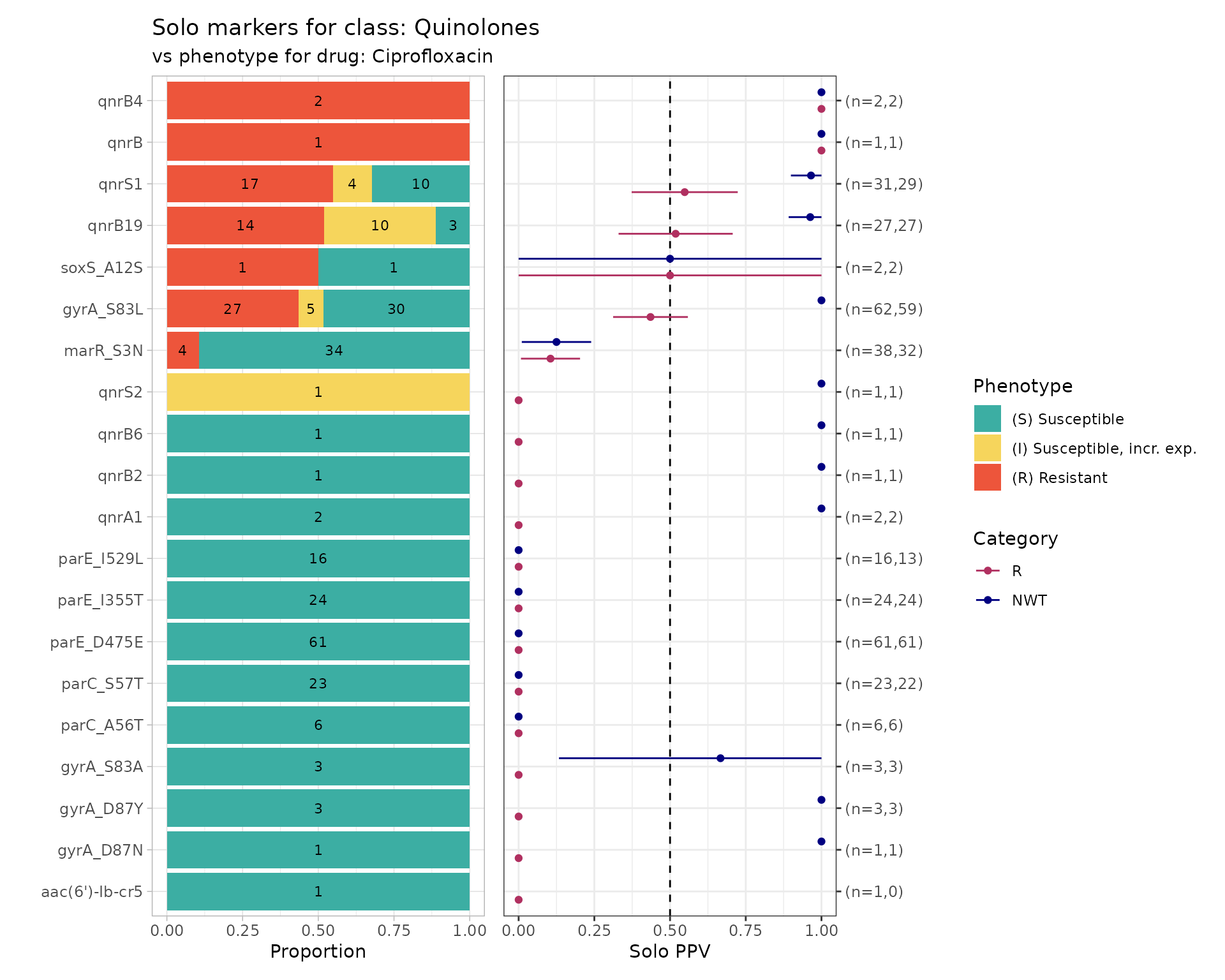
# Output table
soloPPV_cipro$solo_stats
#> # A tibble: 40 × 8
#>    marker         category     x     n   ppv    se ci.lower ci.upper
#>    <chr>          <chr>    <dbl> <int> <dbl> <dbl>    <dbl>    <dbl>
#>  1 aac(6')-Ib-cr5 R            0     1     0     0        0        0
#>  2 gyrA_D87N      R            0     1     0     0        0        0
#>  3 gyrA_D87Y      R            0     3     0     0        0        0
#>  4 gyrA_S83A      R            0     3     0     0        0        0
#>  5 parC_A56T      R            0     6     0     0        0        0
#>  6 parC_S57T      R            0    23     0     0        0        0
#>  7 parE_D475E     R            0    61     0     0        0        0
#>  8 parE_I355T     R            0    24     0     0        0        0
#>  9 parE_I529L     R            0    16     0     0        0        0
#> 10 qnrA1          R            0     2     0     0        0        0
#> # ℹ 30 more rows

# Interim matrices with data used to compute stats and plots
soloPPV_cipro$solo_binary
#> # A tibble: 306 × 9
#>    id           pheno ecoff   mic  disk     R   NWT marker    value
#>    <chr>        <sir> <sir> <mic> <dsk> <dbl> <dbl> <chr>     <dbl>
#>  1 SAMN03177618   S    NWT   0.25    NA     0     1 gyrA_S83L     1
#>  2 SAMN03177619   S    NWT   0.12    NA     0     1 gyrA_D87Y     1
#>  3 SAMN03177623   S    NWT   0.25    NA     0     1 gyrA_S83L     1
#>  4 SAMN03177631   S    NWT   0.25    NA     0     1 gyrA_S83L     1
#>  5 SAMN03177635   S    NWT   0.25    NA     0     1 gyrA_S83L     1
#>  6 SAMN03177637   S    NWT   0.25    NA     0     1 gyrA_S83L     1
#>  7 SAMN03177638   S    NWT   0.25    NA     0     1 qnrB6         1
#>  8 SAMN03177639   S    NWT   0.12    NA     0     1 gyrA_S83L     1
#>  9 SAMN03177643   S    NWT   0.25    NA     0     1 gyrA_S83L     1
#> 10 SAMN03177646   S    NWT   0.25    NA     0     1 gyrA_S83L     1
#> # ℹ 296 more rows

soloPPV_cipro$amr_binary
#> # A tibble: 3,629 × 51
#>    id        pheno ecoff     mic  disk     R   NWT gyrA_S83L gyrA_D87Y gyrA_D87N
#>    <chr>     <sir> <sir>   <mic> <dsk> <dbl> <dbl>     <dbl>     <dbl>     <dbl>
#>  1 SAMN0317…   S     WT  <=0.015    NA     0     0         0         0         0
#>  2 SAMN0317…   S     WT  <=0.015    NA     0     0         0         0         0
#>  3 SAMN0317…   S     WT  <=0.015    NA     0     0         0         0         0
#>  4 SAMN0317…   S    NWT    0.250    NA     0     1         1         0         0
#>  5 SAMN0317…   S    NWT    0.120    NA     0     1         0         1         0
#>  6 SAMN0317…   S     WT  <=0.015    NA     0     0         0         0         0
#>  7 SAMN0317…   S     WT  <=0.015    NA     0     0         0         0         0
#>  8 SAMN0317…   R    NWT   >4.000    NA     1     1         1         0         1
#>  9 SAMN0317…   S    NWT    0.250    NA     0     1         1         0         0
#> 10 SAMN0317…   R    NWT   >4.000    NA     1     1         1         0         1
#> # ℹ 3,619 more rows
#> # ℹ 41 more variables: parC_S80I <dbl>, parE_S458A <dbl>, parC_S80R <dbl>,
#> #   parE_L416F <dbl>, qnrB6 <dbl>, gyrA_D87G <dbl>, parC_S57T <dbl>,
#> #   parC_E84A <dbl>, soxS_A12S <dbl>, qnrB2 <dbl>, qnrS2 <dbl>,
#> #   parC_E84K <dbl>, parC_A56T <dbl>, qnrB19 <dbl>, `aac(6')-Ib-cr5` <dbl>,
#> #   parC_E84V <dbl>, parE_I529L <dbl>, parE_S458T <dbl>, parE_E460D <dbl>,
#> #   parC_E84G <dbl>, qnrS1 <dbl>, marR_S3N <dbl>, `aac(6')-Ib-cr` <dbl>, …
9. Compare markers with assay data
So far we have considered only the impact of individual markers, and their association with categorical S/I/R or WT/NWT calls.
UpSet plots
The function amr_upset() takes as binary matrix table
cip_bin summarising ciprofloxacin resistance vs quinolone
markers, generated using get_binary_matrix(), and explores
the distribution of MIC or disk diffusion assay values for all observed
combinations of markers (solo or multiple markers). It visualises the
data in the form of an upset plot, showing the distribution of assay
values and S/I/R calls for each observed marker combination, and returns
a summary of these distributions (including sample size, median and
interquartile range, number and proportion classified as R).
The function returns 2 objects:
summary: data frame containing summarising the data associated with each combination of markersplot: an upset plot showing the distribution of assay values, and breakdown of S/I/R calls, for each observed marker combination
# Compare ciprofloxacin MIC data with quinolone marker combinations,
#    using the binary matrix we constructed earlier via get_binary_matrix()
cipro_mic_upset <- amr_upset(
  cip_bin,
  min_set_size = 2,
  assay = "mic",
  order = "value"
)
#> Ordering markers by frequency
#> Scale for y is already present.
#> Adding another scale for y, which will replace the existing scale.
#> Scale for y is already present.
#> Adding another scale for y, which will replace the existing scale.
# Output table
cipro_mic_upset$summary
#> # A tibble: 103 × 21
#>    marker_list        marker_count     n combination_id   R.n   R.ppv R.ci_lower
#>    <chr>                     <dbl> <int> <fct>          <dbl>   <dbl>      <dbl>
#>  1 ""                            0  2590 0_0_0_0_0_0_0…    10 0.00386    0.00147
#>  2 "qnrB"                        1     1 0_0_0_0_0_0_0…     1 1          1
#>  3 "parE_E460K, gyrA…            2     1 0_0_0_0_0_0_0…     1 1          1
#>  4 "parE_D475E"                  1    61 0_0_0_0_0_0_0…     0 0          0
#>  5 "qnrA1"                       1     2 0_0_0_0_0_0_0…     0 0          0
#>  6 "gyrA_S83A"                   1     3 0_0_0_0_0_0_0…     0 0          0
#>  7 "qnrB4"                       1     2 0_0_0_0_0_0_0…     2 1          1
#>  8 "parE_I355T"                  1    24 0_0_0_0_0_0_0…     0 0          0
#>  9 "marR_S3N"                    1    38 0_0_0_0_0_0_0…     4 0.105      0.00769
#> 10 "marR_S3N, parE_D…            2     4 0_0_0_0_0_0_0…     0 0          0
#> # ℹ 93 more rows
#> # ℹ 14 more variables: R.ci_upper <dbl>, R.denom <int>, NWT.n <dbl>,
#> #   NWT.ppv <dbl>, NWT.ci_lower <dbl>, NWT.ci_upper <dbl>, NWT.denom <int>,
#> #   median_excludeRangeValues <dbl>, q25_excludeRangeValues <dbl>,
#> #   q75_excludeRangeValues <dbl>, n_excludeRangeValues <int>,
#> #   median_ignoreRanges <dbl>, q25_ignoreRanges <dbl>, q75_ignoreRanges <dbl>
PPV plots
The function amr_ppv() uses the same underlying approach
as amr_upset() but transposes the orientation of the data
so it looks more like the solo_ppv() plot but for
combinations of markers as well as those found solo.
Like amr_upset it takes as binary matrix table
cip_bin summarising ciprofloxacin resistance vs quinolone
markers, generated using get_binary_matrix(), and creates a
multi-panel plot and summary statistics table.
The left-most panel indicates which marker/combinations are shown in
each row of the plot, either as a list of marker names (default) or as
an upset-style grid (set upset_grid=TRUE to turn this
on).
The other panels available are
category plot: stacked bar plot showing S/I/R calls (ON by default, set plot_category=
FALSEto turn this off)PPV plot: forest-style plot showing point estimates for R/NWT PPV, with horizontal lines indicating 95% confidence intervals (ON by default, set plot_ppv=
FALSEto turn this off)assay plot: boxplot of assay (MIC/disk) values (OFF by default, set plot_assay=
TRUEand assay="mic"or assay="disk"to turn this on)
The function returns 2 objects:
summary: data frame containing summarising the data associated with each combination of markersplot: an upset plot showing the distribution of assay values, and breakdown of S/I/R calls, for each observed marker combination
# Default plot
cipro_mic_ppv <- amr_ppv(
  cip_bin,
  min_set_size = 10,
  upset_grid = T
)
#> Ordering markers by frequency
#> Scale for y is already present.
#> Adding another scale for y, which will replace the existing scale.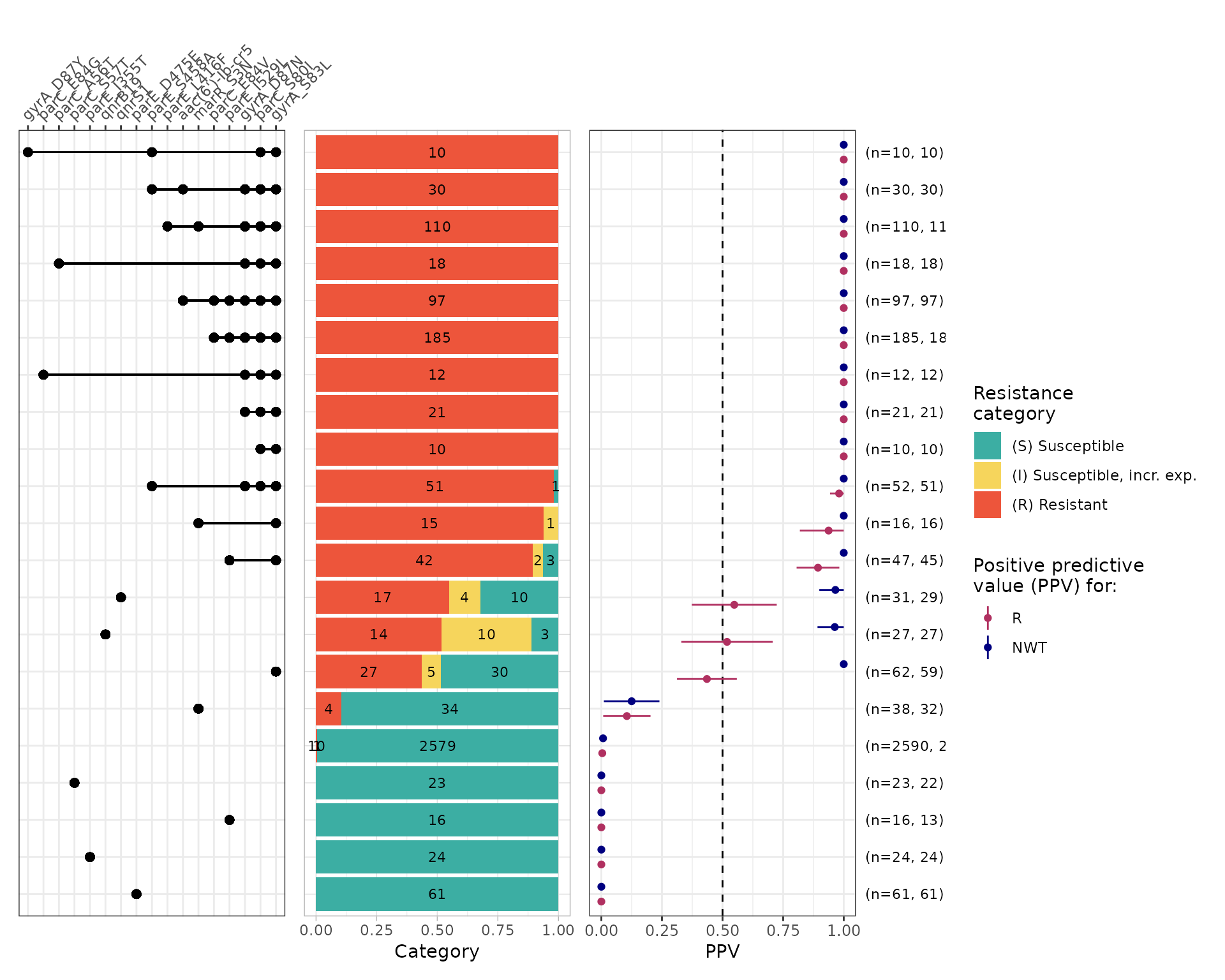
# add MIC, remove category plot, label rows with marker list
cipro_mic_ppv2 <- amr_ppv(
  cip_bin,
  min_set_size = 10,
  upset_grid = F,
  plot_assay = T, assay = "mic",
  plot_category = F
)
#> Ordering markers by frequency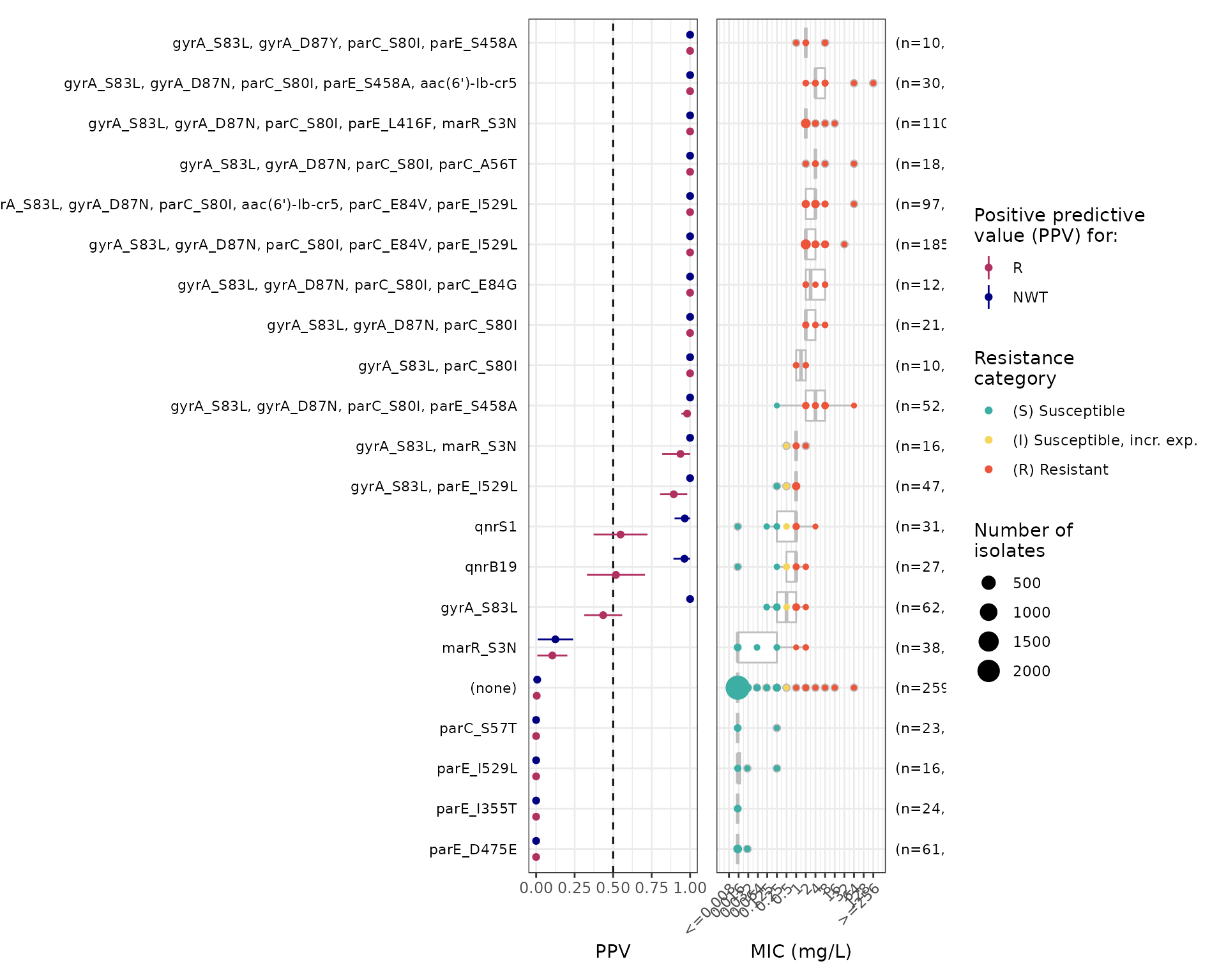
# Output table
cipro_mic_ppv$summary
#> # A tibble: 103 × 14
#>    marker_list        marker_count     n combination_id   R.n   R.ppv R.ci_lower
#>    <chr>                     <dbl> <int> <fct>          <dbl>   <dbl>      <dbl>
#>  1 ""                            0  2590 0_0_0_0_0_0_0…    10 0.00386    0.00147
#>  2 "qnrB"                        1     1 0_0_0_0_0_0_0…     1 1          1
#>  3 "parE_E460K, gyrA…            2     1 0_0_0_0_0_0_0…     1 1          1
#>  4 "parE_D475E"                  1    61 0_0_0_0_0_0_0…     0 0          0
#>  5 "qnrA1"                       1     2 0_0_0_0_0_0_0…     0 0          0
#>  6 "gyrA_S83A"                   1     3 0_0_0_0_0_0_0…     0 0          0
#>  7 "qnrB4"                       1     2 0_0_0_0_0_0_0…     2 1          1
#>  8 "parE_I355T"                  1    24 0_0_0_0_0_0_0…     0 0          0
#>  9 "marR_S3N"                    1    38 0_0_0_0_0_0_0…     4 0.105      0.00769
#> 10 "marR_S3N, parE_D…            2     4 0_0_0_0_0_0_0…     0 0          0
#> # ℹ 93 more rows
#> # ℹ 7 more variables: R.ci_upper <dbl>, R.denom <int>, NWT.n <dbl>,
#> #   NWT.ppv <dbl>, NWT.ci_lower <dbl>, NWT.ci_upper <dbl>, NWT.denom <int>