Example exploring gene vs mutation combinations
Kara Tsang
Source:vignettes/KlebsiellaMultipleGenotypers.Rmd
KlebsiellaMultipleGenotypers.RmdAnalysing meropenem resistance Klebsiella pneumoniae
This vignette demonstrates an example of how to investigate associations between Klebsiella pneumoniae meropenem antibiotic susceptibility testing (AST) data and AMR genotype data (Kleborate, AMRFinderPlus and RGI), including examining the orthogonal effects of acquired carbapenemase genes and porin mutations.
We will be using the AST data and AMR genotyping outputs for n=1490 isolates from the European Survey of Carbapenemase-Producing Enterobacteriaceae (EuSCAPE) published as ‘Epidemic of carbapenem-resistant Klebsiella pneumoniae in Europe is driven by nosocomial spread’ by David, S., et al. Nature Microbiology, 2016.
Whole genome sequence reads were downloaded from NCBI Bioproject PRJEB10018 / European Nucleotide Archive ERP011196, trimmed using Trim Galore v0.5.0, and assembled using Unicycler v0.5.0. The assembled genomes were then run through each AMR genotyper:
- Kleborate v3.1.3
- Kleborate version development branch - commit #4ec1dcb on March 17, 2026
- Resistance Gene Idenfier (RGI v6.0.6) - using the Comprehensive Antibiotic Resistance Database (CARD, v4.0.1)
AMRFinderPlus results were generated by EMBL-EBI Antimicrobial Resistance Portal using - AMRFinderPlus v4.0 with NCBI Reference Gene Catalog database version 2025-07-16.1.
Phenotype Data
The download_ebi() function lets you load phenotype data
and interpret susceptible, intermediate, and resistant phenotypes using
EUCAST breakpoints and ECOFF. A copy of the data objected produced below
is available in the AMRgen package as kp_mero_euscape.
# Download Klebsiella pneumoniae AST data from EBI, filtering for meropenem and re-interpret with EUCAST breakpoints and ECOFF

kp_mero <- download_ebi(
  pheno_drug = "meropenem",
  species = "Klebsiella pneumoniae",
  reformat = TRUE,
  interpret_eucast = TRUE,
  interpret_ecoff = TRUE
)

# Filter for isolates in EuSCAPE paper (PMID: 31358985)
kp_mero_euscape <- kp_mero %>% filter(grepl("31358985", source))

# There are assemblies from NCBI that are flagged for contamination and supposed to be excluded. For example, see SAMEA3729690 (https://www.ncbi.nlm.nih.gov/datasets/genome/?biosample=SAMEA3729690)

contaminated_assemblies <- c("SAMEA3729690", "SAMEA3721062", "SAMEA3721052", "SAMEA3720966", "SAMEA3673128", "SAMEA3538742", "SAMEA3721188", "SAMEA3649589", "SAMEA3538652", "SAMEA3649503", "SAMEA3538911", "SAMEA3727711", "SAMEA3649452", "SAMEA3649453", "SAMEA3649454", "SAMEA3649467", "SAMEA3721063", "SAMEA3538862", "SAMEA3538667", "SAMEA3673004", "SAMEA3729818", "SAMEA3729660", "SAMEA3673078", "SAMEA3673097")

# Remove contaminated assemblies from phenotype list
kp_mero_euscape <- kp_mero_euscape %>%
  filter(!id %in% contaminated_assemblies)
Check the data frame
head(kp_mero_euscape)
#> # A tibble: 6 × 43
#>   id        drug   mic  disk pheno_provided pheno_eucast ecoff guideline method
#>   <chr>     <ab> <mic> <dsk> <sir>          <sir>        <sir> <chr>     <chr>
#> 1 SAMEA372… MEM   2.00    NA   NA             S           NWT  NA        broth …
#> 2 SAMEA372… MEM   4.00    NA   NA             I           NWT  NA        broth …
#> 3 SAMEA372… MEM   0.12    NA   NA             S            WT  NA        broth …
#> 4 SAMEA372… MEM   1.00    NA   NA             S           NWT  NA        broth …
#> 5 SAMEA372… MEM   4.00    NA   NA             I           NWT  NA        broth …
#> 6 SAMEA372… MEM   8.00    NA   NA             I           NWT  NA        broth …
#> # ℹ 34 more variables: platform <chr>, source <chr>, spp_pheno <mo>,
#> #   SRA_accession <chr>, assembly_ID <chr>, collection_year <int>,
#> #   ISO_country_code <chr>, host <chr>, host_age <chr>, host_sex <chr>,
#> #   isolate <chr>, isolation_source <chr>, isolation_source_category <chr>,
#> #   isolation_latitude <chr>, isolation_longitude <chr>, genus <chr>,
#> #   organism <chr>, Updated_phenotype_CLSI <chr>,
#> #   Updated_phenotype_EUCAST <chr>, used_ECOFF <chr>, database <chr>, …
Phenotype Data Summary
Summarize the downloaded phenotype data and plot the minimum inhibitory concentration (MIC) distributions with EUCAST breakpoints and ECOFF.
# Summary of meropenem phenotype data including S/I/R count using EUCAST breakpoint and ECOFF
summarise_pheno(kp_mero_euscape, pheno_cols = c("pheno_eucast", "ecoff"))
#> $uniques
#> # A tibble: 7 × 2
#>   column    n_unique
#>   <chr>        <int>
#> 1 id            1490
#> 2 drug             1
#> 3 spp_pheno        1
#> 4 method           1
#> 5 platform         1
#> 6 guideline        1
#> 7 source           2
#>
#> $drugs
#> # A tibble: 1 × 4
#>   drug drug_name spp_pheno               mic
#>   <ab> <chr>     <chr>                 <int>
#> 1 MEM  Meropenem Klebsiella pneumoniae  1490
#>
#> $details
#> # A tibble: 2 × 8
#>   drug drug_name spp_pheno             method    platform guideline source   mic
#>   <ab> <chr>     <chr>                 <chr>     <chr>    <chr>     <chr>  <int>
#> 1 MEM  Meropenem Klebsiella pneumoniae broth di… NA       NA        31358…   628
#> 2 MEM  Meropenem Klebsiella pneumoniae broth di… NA       NA        31358…   862
#>
#> $pheno_counts_list
#> $pheno_counts_list$pheno_eucast
#> # A tibble: 1 × 6
#>   drug drug_name spp_pheno                 S     I     R
#>   <ab> <chr>     <chr>                 <int> <int> <int>
#> 1 MEM  Meropenem Klebsiella pneumoniae   973   126   391
#>
#> $pheno_counts_list$ecoff
#> # A tibble: 1 × 5
#>   drug drug_name spp_pheno                WT   NWT
#>   <ab> <chr>     <chr>                 <int> <int>
#> 1 MEM  Meropenem Klebsiella pneumoniae   710   780

# MIC distribution coloured by phenotype interpretation using EUCAST breakpoint
assay_by_var(
  pheno_table = kp_mero_euscape,
  pheno_drug = "Meropenem",
  measure = "mic",
  colour_by = "pheno_eucast",
  species = "Klebsiella pneumoniae"
)
#>   MIC breakpoints determined using AMR package: S <= 2 and R > 8
#>   NOTE: Multiple breakpoint entries, for different sites: Non-meningitis; Meningitis. Using the one with the highest S breakpoint (Non-meningitis).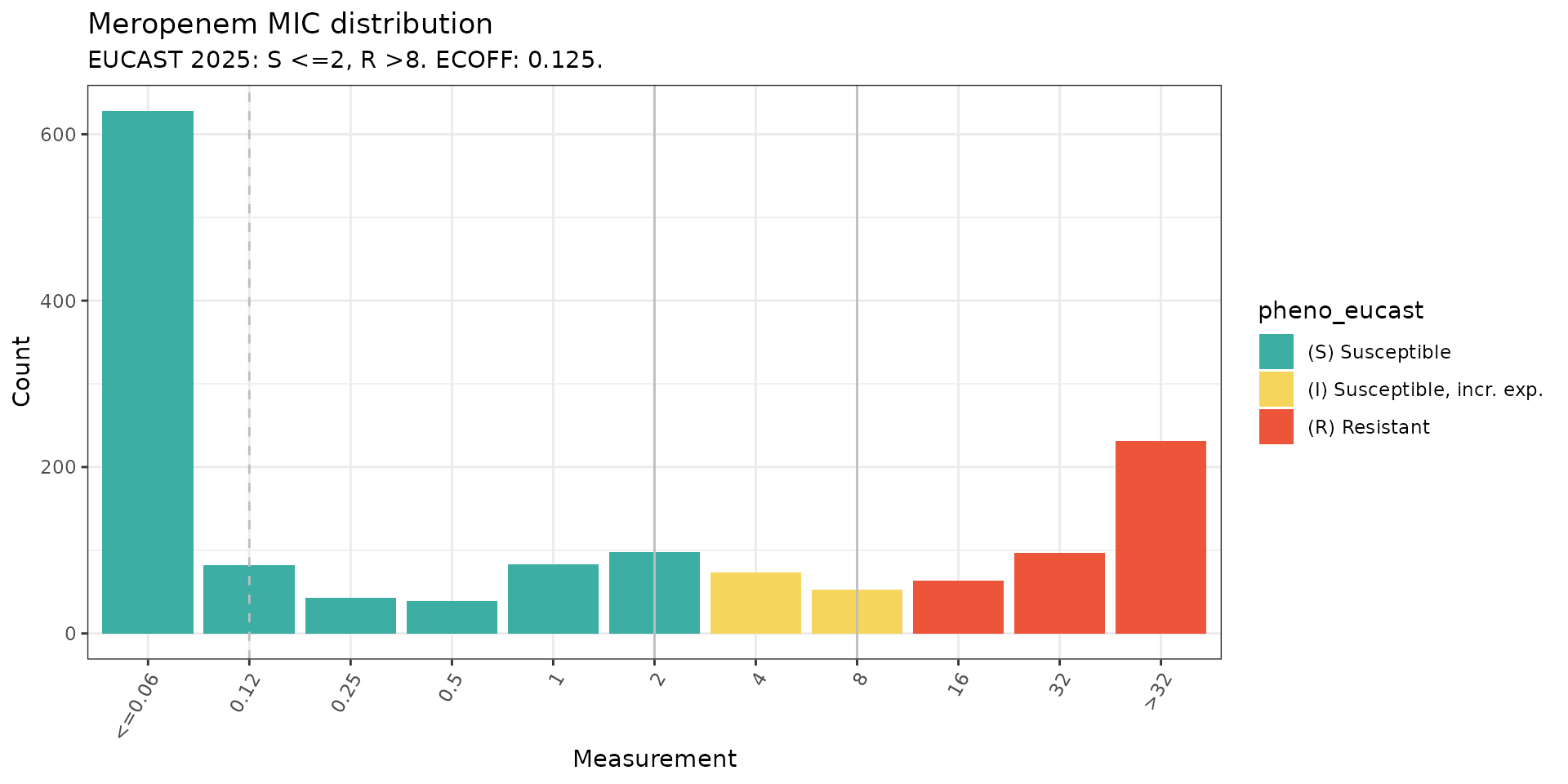
# Summary of meropenem phenotypes using ECOFF
kp_mero_euscape %>% count(ecoff)
#> # A tibble: 2 × 2
#>   ecoff     n
#>   <sir> <int>
#> 1   WT    710
#> 2  NWT    780

# MIC distribution coloured by ECOFF
assay_by_var(
  pheno_table = kp_mero_euscape,
  pheno_drug = "Meropenem",
  measure = "mic",
  colour_by = "ecoff",
  species = "Klebsiella pneumoniae"
)
#>   MIC breakpoints determined using AMR package: S <= 2 and R > 8
#>   NOTE: Multiple breakpoint entries, for different sites: Non-meningitis; Meningitis. Using the one with the highest S breakpoint (Non-meningitis).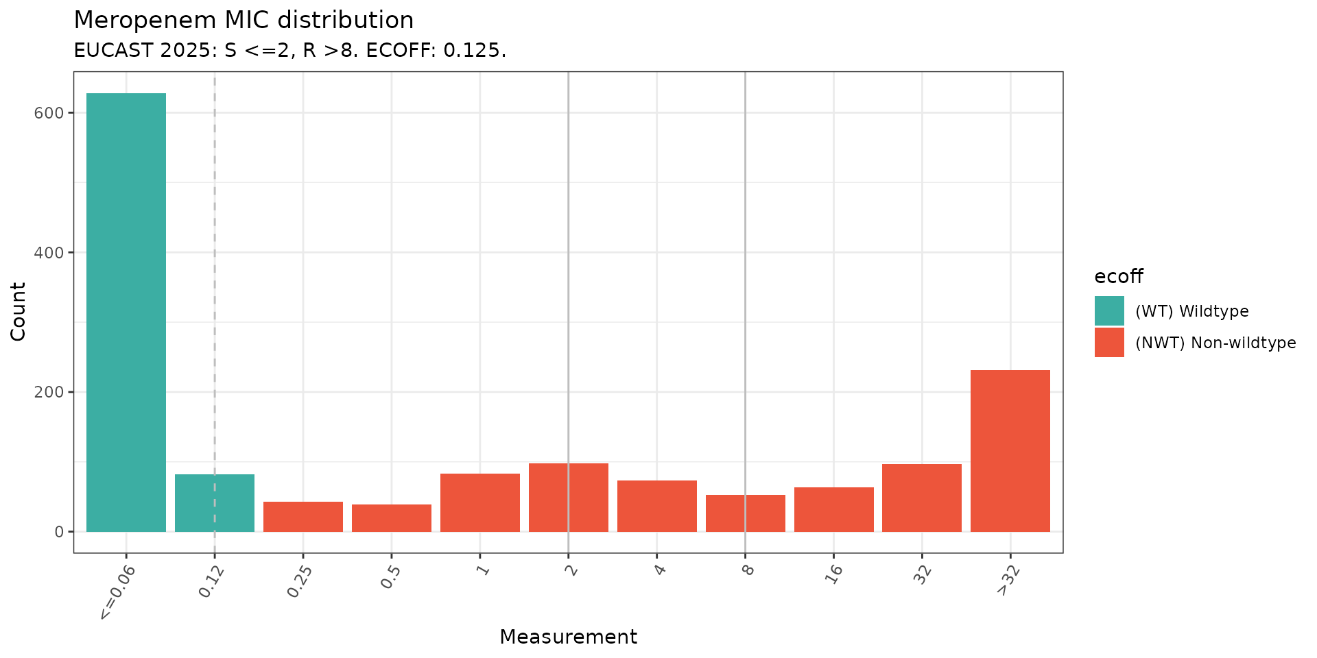
Genotypes from Kleborate
Kleborate screens Klebsiella pneumoniae species complex (KpSC) genome assemblies to identify sequence types (MLST), species, antimicrobial resistance (AMR) genes, virulence loci (e.g., yersiniabactin, aerobactin), and capsule/LPS serotypes (K and O antigens), published here. It can be run on the command line or via Pathogenwatch.
Import Kleborate Genotype Data
The import_kleborate() function imports the output table
from Kleborate,
extracts the AMR genotyping data, and formats it to be used with AMRgen
functions.
Mutation notation in Kleborate changed after v3.1.3 to adhere to HGVS Nomenclature, so:
To import Kleborate output <=v3.1.3 (using informal nomenclature (e.g. [gene]-[mutation], [gene]-X%, OmpK36GD)), in the
import_kleborate()function, sethgvs = FALSE.To import Kleborate output >v3.1.3 (using HGVS Nomenclature), in the
import_kleborate()function, set tohgvs=TRUE(which is already the default option).
We are importing the latest version of Kleborate which is in the development branch - commit #4ec1dcb from March 17, 2026. This version uses HGVS Nomenclature for describing mutations and includes an updated AMR database compared to the most recent Kleborate release v3.2.4.
A table of Kleborate results generated for the EuSCAPE genomes is
available in the AMRgen package as kleborate_raw. Let’s
import this to AMRgen genotype table format and summarise the
content:
# Updated Kleborate results from the development branch as of March 17, 2026 (commit #4ec1dcb)
head(kleborate_raw, n = 10)
#> # A tibble: 10 × 122
#>    strain    species species_match contig_count    N50 largest_contig total_size
#>    <chr>     <chr>   <chr>                <dbl>  <dbl>          <dbl>      <dbl>
#>  1 SAMEA349… Klebsi… strong                 141 230759         470757    5578320
#>  2 SAMEA349… Klebsi… strong                  88 370309         938079    5384685
#>  3 SAMEA349… Klebsi… strong                  90 238750         529125    5446454
#>  4 SAMEA349… Klebsi… strong                 144 207582         663698    5574298
#>  5 SAMEA349… Klebsi… strong                 142 263498         678692    5486238
#>  6 SAMEA349… Klebsi… strong                  79 285199         991412    5529803
#>  7 SAMEA349… Klebsi… strong                 280 178980         585359    5817055
#>  8 SAMEA349… Klebsi… strong                 108 209418         517450    5379124
#>  9 SAMEA349… Klebsi… strong                 134 371444         984005    5558705
#> 10 SAMEA349… Klebsi… strong                 142 197944         636773    5497421
#> # ℹ 115 more variables: GC_content <dbl>, ambiguous_bases <chr>,
#> #   QC_warnings <chr>, ST <chr>, gapA <dbl>, infB <dbl>, mdh <dbl>, pgi <dbl>,
#> #   phoE <dbl>, rpoB <dbl>, tonB <dbl>, YbST <chr>, Yersiniabactin <chr>,
#> #   ybtS <chr>, ybtX <chr>, ybtQ <chr>, ybtP <chr>, ybtA <chr>, irp2 <chr>,
#> #   irp1 <chr>, ybtU <chr>, ybtT <chr>, ybtE <chr>, fyuA <chr>,
#> #   spurious_ybt_hits <chr>, CbST <chr>, Colibactin <chr>, clbA <chr>,
#> #   clbB <chr>, clbC <chr>, clbD <chr>, clbE <chr>, clbF <chr>, clbG <chr>, …

# Import Kleborate
kleborate_dev <- import_kleborate(kleborate_raw)

# View summary of genotypes
summarise_geno(kleborate_dev)
#> $uniques
#> # A tibble: 6 × 2
#>   column         n_unique
#>   <chr>             <int>
#> 1 id                 1490
#> 2 marker              470
#> 3 drug                  1
#> 4 drug_class           13
#> 5 gene                293
#> 6 variation type        4
#>
#> $per_type
#> # A tibble: 4 × 6
#>   `variation type`                  id marker  drug drug_class  gene
#>   <chr>                          <int>  <int> <int>      <int> <int>
#> 1 Gene presence detected          1490    288     1         13   288
#> 2 Inactivating mutation detected   569    167     1          2     3
#> 3 Nucleotide variant detected       15      1     1          1     1
#> 4 Protein variant detected         874     14     1          2     3
#>
#> $drugs
#> # A tibble: 13 × 5
#>    drug  drug_class                markers samples  hits
#>    <lgl> <chr>                       <int>   <int> <int>
#>  1 NA    Aminoglycosides                68    1060  2709
#>  2 NA    Beta-lactams                   76    1457  2833
#>  3 NA    Carbapenems                   153     770  1477
#>  4 NA    Cephalosporins (3rd gen.)      18     648   668
#>  5 NA    Macrolides                     15     460   924
#>  6 NA    Phenicols                      16     479   572
#>  7 NA    Phosphonics                    17    1485  1490
#>  8 NA    Polymyxins                     33     138   138
#>  9 NA    Quinolones                     26    1021  2665
#> 10 NA    Rifamycins                      3     119   128
#> 11 NA    Sulfonamides                   13     917  1096
#> 12 NA    Tetracyclines                  12     514   554
#> 13 NA    Trimethoprims                  21     941  1110
#>
#> $markers
#> # A tibble: 471 × 5
#>    marker   drug  drug_class                `variation type`           n
#>    <chr>    <lgl> <chr>                     <chr>                  <int>
#>  1 ACC-4.v1 NA    Beta-lactams              Gene presence detected     2
#>  2 CMY-13   NA    Beta-lactams              Gene presence detected     1
#>  3 CMY-16   NA    Beta-lactams              Gene presence detected    31
#>  4 CMY-2.v2 NA    Beta-lactams              Gene presence detected     1
#>  5 CMY-30   NA    Cephalosporins (3rd gen.) Gene presence detected     1
#>  6 CMY-4.v1 NA    Beta-lactams              Gene presence detected     5
#>  7 CMY-6    NA    Beta-lactams              Gene presence detected     2
#>  8 CTX-M-1  NA    Cephalosporins (3rd gen.) Gene presence detected     1
#>  9 CTX-M-14 NA    Cephalosporins (3rd gen.) Gene presence detected    16
#> 10 CTX-M-15 NA    Cephalosporins (3rd gen.) Gene presence detected   568
#> # ℹ 461 more rows
Kleborate Genotype and Phenotype Summary
Summarize how many markers are associated with the beta-lactam and carbapenem drug class since Kleborate only operates at a drug class level.
summarise_geno_pheno(kleborate_dev, kp_mero_euscape,
  pheno_cols = c("pheno_eucast", "ecoff")
)
#> $overlapping_samples
#> [1] 1490
#>
#> $drugs_with_pheno
#> # A tibble: 2 × 6
#>   drug     n drug_class   drug_name spp_pheno               mic
#>   <ab> <int> <chr>        <chr>     <chr>                 <int>
#> 1 MEM   1490 Carbapenems  Meropenem Klebsiella pneumoniae  1490
#> 2 MEM   1490 Beta-lactams Meropenem Klebsiella pneumoniae  1490
#>
#> $geno_hits
#> # A tibble: 2 × 6
#>   drug  drug_name drug_class   markers samples  hits
#>   <lgl> <chr>     <chr>          <int>   <int> <int>
#> 1 NA    NA        Beta-lactams      76    1457  2833
#> 2 NA    NA        Carbapenems      153     770  1477
#>
#> $geno_markers
#> # A tibble: 229 × 6
#>    marker   drug  drug_name drug_class   `variation type`           n
#>    <chr>    <lgl> <chr>     <chr>        <chr>                  <int>
#>  1 ACC-4.v1 NA    NA        Beta-lactams Gene presence detected     2
#>  2 CMY-13   NA    NA        Beta-lactams Gene presence detected     1
#>  3 CMY-16   NA    NA        Beta-lactams Gene presence detected    31
#>  4 CMY-2.v2 NA    NA        Beta-lactams Gene presence detected     1
#>  5 CMY-4.v1 NA    NA        Beta-lactams Gene presence detected     5
#>  6 CMY-6    NA    NA        Beta-lactams Gene presence detected     2
#>  7 CTX-M-33 NA    NA        Carbapenems  Gene presence detected     1
#>  8 DHA-1    NA    NA        Beta-lactams Gene presence detected    78
#>  9 IMP-1    NA    NA        Carbapenems  Gene presence detected     3
#> 10 KPC-12   NA    NA        Carbapenems  Gene presence detected     1
#> # ℹ 219 more rows
#>
#> $pheno_counts_list
#> $pheno_counts_list$ecoff
#> # A tibble: 1 × 5
#>   drug drug_name spp_pheno                WT   NWT
#>   <ab> <chr>     <chr>                 <int> <int>
#> 1 MEM  Meropenem Klebsiella pneumoniae   710   780
#>
#> $pheno_counts_list$pheno_eucast
#> # A tibble: 1 × 6
#>   drug drug_name spp_pheno                 S     I     R
#>   <ab> <chr>     <chr>                 <int> <int> <int>
#> 1 MEM  Meropenem Klebsiella pneumoniae   973   126   391
Phenotypes vs Kleborate Genotypes
Generate Binary Matrix for Kleborate AMR Markers
Most AMRgen analysis functions require a binary matrix with one
sample per row, and columns indicating the phenotype and genotype data
in columns, where a 1 indicates the presence and
0 indicates the absence of the phenotype or genotypic
marker in that sample. This is produced using the
get_binary_matrix function:
kleborate_binary_matrix <- get_binary_matrix(
  geno_table = kleborate_dev,
  pheno_table = kp_mero_euscape,
  pheno_drug = "Meropenem",
  geno_class = c("Carbapenems"),
  sir_col = "pheno_eucast",
  keep_assay_values = TRUE,
  keep_assay_values_from = "mic",
  marker_col = "marker.label"
)
#>  Defining NWT in binary matrix using ecoff column provided: ecoff

head(kleborate_binary_matrix, n = 10)
#> # A tibble: 10 × 24
#>    id    pheno ecoff    mic     R   NWT `OmpK36..-` `OmpK35..-` `NDM-1` `OXA-48`
#>    <chr> <sir> <sir>  <mic> <dbl> <dbl>       <dbl>       <dbl>   <dbl>    <dbl>
#>  1 SAME…   I    NWT    4.00     0     1           1           0       0        0
#>  2 SAME…   S     WT  <=0.06     0     0           0           0       0        0
#>  3 SAME…   S    NWT    1.00     0     1           1           1       0        0
#>  4 SAME…   I    NWT    4.00     0     1           1           0       0        0
#>  5 SAME…   I    NWT    4.00     0     1           1           1       0        0
#>  6 SAME…   S     WT  <=0.06     0     0           0           0       0        0
#>  7 SAME…   S     WT  <=0.06     0     0           0           0       0        0
#>  8 SAME…   S    NWT    2.00     0     1           1           0       0        0
#>  9 SAME…   S     WT  <=0.06     0     0           0           0       0        0
#> 10 SAME…   S    NWT    0.50     0     1           1           0       0        0
#> # ℹ 14 more variables: `OmpK36..c.25C>T` <dbl>, `KPC-3` <dbl>,
#> #   OmpK36..p.134_135insGD <dbl>, `KPC-2` <dbl>, OmpK36..p.135_136insD <dbl>,
#> #   `OXA-204` <dbl>, `VIM-1` <dbl>, OmpK36..p.136_137insTD <dbl>,
#> #   `VIM-4` <dbl>, `KPC-12` <dbl>, `OXA-232` <dbl>, `CTX-M-33` <dbl>,
#> #   `OXA-162` <dbl>, `IMP-1` <dbl>
Solo PPV Analysis for Kleborate AMR Markers
To understand the individual contribution of an AMR marker found
“solo” (i.e., in the absence of another carbapenem resistance
determinant), we use the solo_ppv() function. The
combined_plot is a visual representation of each AMR marker
found solo, the phenotypic distribution of isolates, and the positive
predictive values (PPVs). The solo_stats table provides the
PPVs, standard error (se), lower confidence interval
(ci.lower), and upper confidence interval
(ci.upper).
soloPPV_kleborate_mero <- solo_ppv(binary_matrix = kleborate_binary_matrix)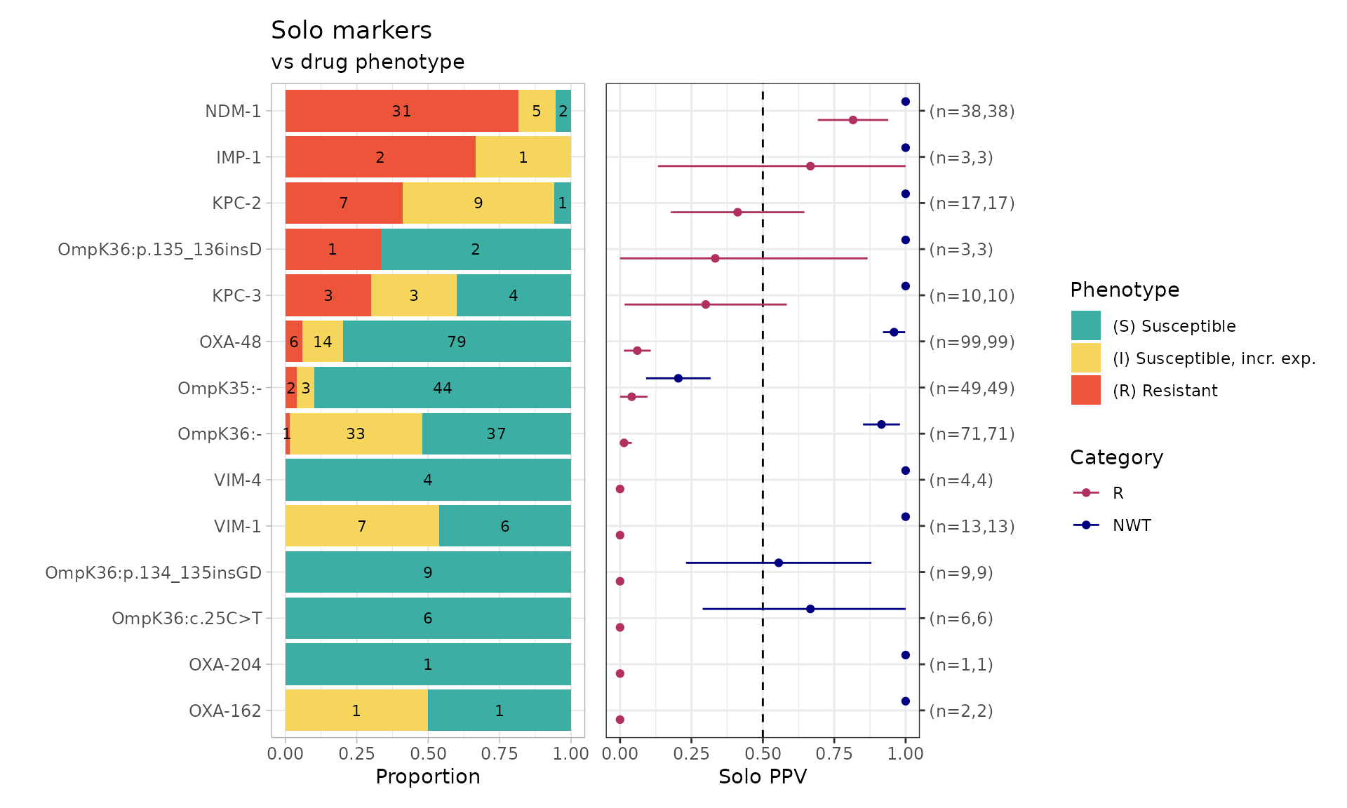
soloPPV_kleborate_mero$solo_stats
#> # A tibble: 28 × 8
#>    marker                category     x     n    ppv     se ci.lower ci.upper
#>    <chr>                 <chr>    <dbl> <int>  <dbl>  <dbl>    <dbl>    <dbl>
#>  1 OXA-162               R            0     2 0      0        0        0
#>  2 OXA-204               R            0     1 0      0        0        0
#>  3 OmpK36:c.25C>T        R            0     6 0      0        0        0
#>  4 OmpK36:p.134_135insGD R            0     9 0      0        0        0
#>  5 VIM-1                 R            0    13 0      0        0        0
#>  6 VIM-4                 R            0     4 0      0        0        0
#>  7 OmpK36:-              R            1    71 0.0141 0.0140   0        0.0415
#>  8 OmpK35:-              R            2    49 0.0408 0.0283   0        0.0962
#>  9 OXA-48                R            6    99 0.0606 0.0240   0.0136   0.108
#> 10 KPC-3                 R            3    10 0.3    0.145    0.0160   0.584
#> # ℹ 18 more rows
Here we can see that the only genotypes whose presence alone, in the absence of any other markers, confers resistance are the carbapenemase genes NDM-1 and IMP-1. Porin mutations alone are not associated with resistance.
Combinatorial PPV Analysis for Kleborate AMR Markers
To understand the contribution of AMR markers found in combination
with one another, we use the amr_ppv() function. The
plot is a visual summary of each AMR marker combination
observed in an UpSet plot format, including phenotypic distribution and
PPVs for each combination. The summary table includes each
AMR marker combination observed, including number of resistant isolates,
positive predictive values, and median assay values (and interquartile
range) where relevant.
comboPPV_kleborate_mero <- amr_ppv(
  binary_matrix = kleborate_binary_matrix,
  order = "value",
  min_set_size = 1,
  pheno_drug = "Meropenem",
  upset_grid = TRUE,
  plot_assay = TRUE,
  assay = "mic"
)
#> Ordering markers by frequency
#> Scale for y is already present.
#> Adding another scale for y, which will replace the existing scale.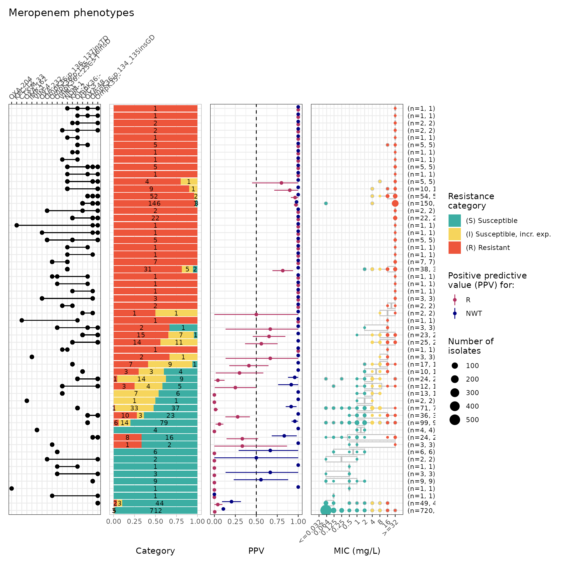
comboPPV_kleborate_mero$summary
#> # A tibble: 56 × 21
#>    marker_list        marker_count     n combination_id   R.n   R.ppv R.ci_lower
#>    <chr>                     <dbl> <int> <fct>          <dbl>   <dbl>      <dbl>
#>  1 ""                            0   720 0_0_0_0_0_0_0…     3 0.00417      0
#>  2 "IMP-1"                       1     3 0_0_0_0_0_0_0…     2 0.667        0.133
#>  3 "OXA-162"                     1     2 0_0_0_0_0_0_0…     0 0            0
#>  4 "VIM-4"                       1     4 0_0_0_0_0_0_0…     0 0            0
#>  5 "VIM-1"                       1    13 0_0_0_0_0_0_0…     0 0            0
#>  6 "OXA-204"                     1     1 0_0_0_0_0_0_0…     0 0            0
#>  7 "OmpK36:p.135_136…            1     3 0_0_0_0_0_0_0…     1 0.333        0
#>  8 "KPC-2"                       1    17 0_0_0_0_0_0_0…     7 0.412        0.178
#>  9 "KPC-2, VIM-1"                2     2 0_0_0_0_0_0_0…     2 1            1
#> 10 "OmpK36:p.134_135…            1     9 0_0_0_0_0_0_1…     0 0            0
#> # ℹ 46 more rows
#> # ℹ 14 more variables: R.ci_upper <dbl>, R.denom <int>, NWT.n <dbl>,
#> #   NWT.ppv <dbl>, NWT.ci_lower <dbl>, NWT.ci_upper <dbl>, NWT.denom <int>,
#> #   median_excludeRangeValues <dbl>, q25_excludeRangeValues <dbl>,
#> #   q75_excludeRangeValues <dbl>, n_excludeRangeValues <int>,
#> #   median_ignoreRanges <dbl>, q25_ignoreRanges <dbl>, q75_ignoreRanges <dbl>
UpSet Plot for Kleborate AMR Markers
Similar to the previous amr_ppv() function, the
amr_upset() function will generate a summary
table and plot that shows the combinations of AMR markers
found in the isolates and their phenotypic distribution. The UpSet
plot produced by amr_upset() is similar to
that generated using amr_ppv() function, but oriented
vertically and without the PPV panel. Restricting the plot to marker
combinations observed at least 3 times in the dataset
(min_set_size=3) makes it a little easier to see what’s
going on.
kp_mic_upset_kleborate <- amr_upset(kleborate_binary_matrix,
  assay = "mic", species = "Klebsiella pneumoniae", min_set_size = 3
)
#> Ordering markers by frequency
#> Scale for y is already present.
#> Adding another scale for y, which will replace the existing scale.
#> Scale for y is already present.
#> Adding another scale for y, which will replace the existing scale.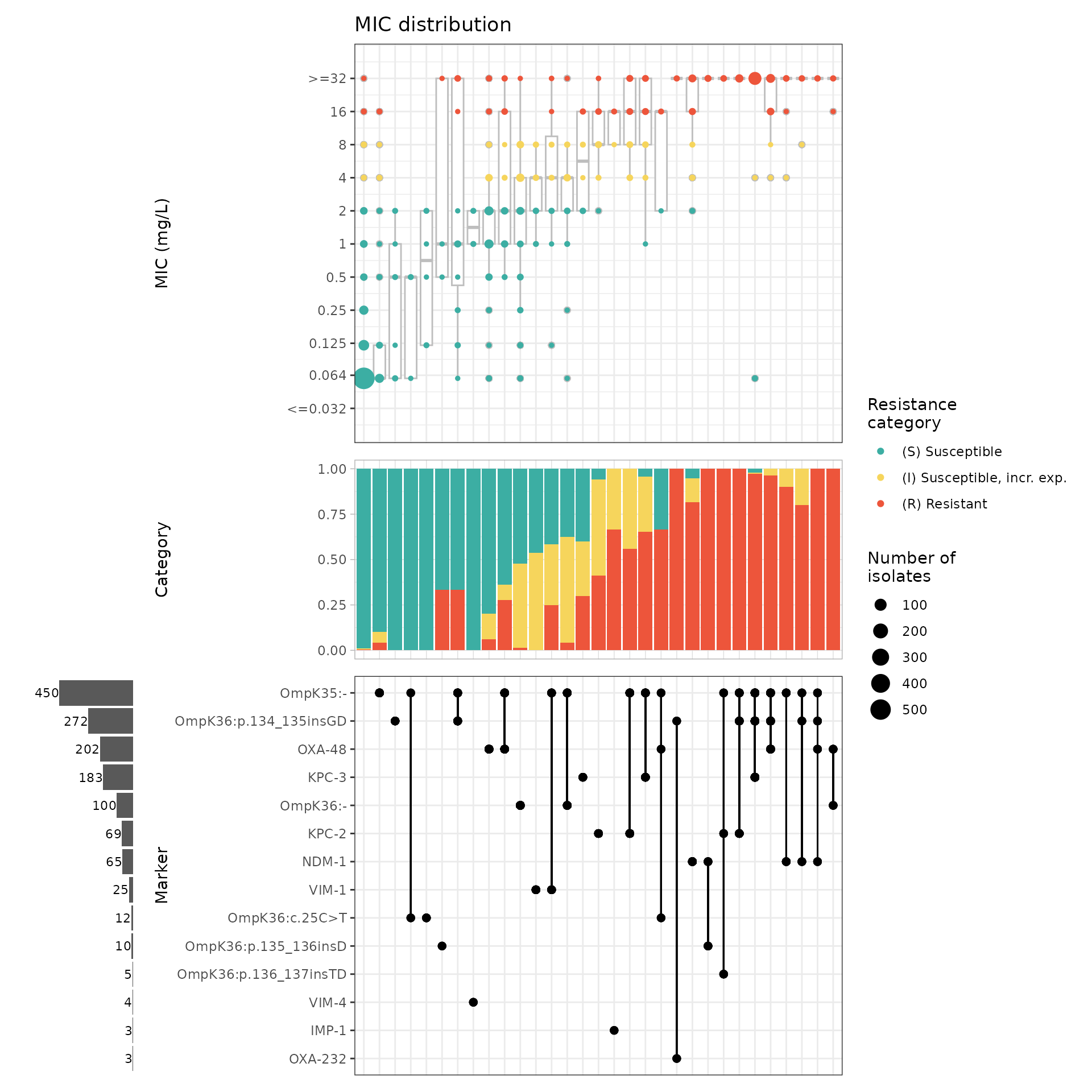
It’s still quite complex to follow the plot and spot patterns, as we have carbapenemase genes mixed in with mutations, making it difficult to compare the effect of a given gene with and without a mutation (and vice versa).
To simplify things, let’s group the various insertion mutations together.
# modify marker labels in the genotype table
kleborate_dev_plotting <- kleborate_dev %>%
  mutate(marker.label = case_when(
    marker.label == "OmpK36:-" ~ "OmpK36Δ",
    marker.label == "OmpK35:-" ~ "OmpK35Δ",
    grepl("OmpK36:p", marker.label) ~ "OmpK36ins",
    TRUE ~ marker.label
  ))

# calculate binary matrix from this updated genotype table, within the amr_upset function
kp_mic_upset_kleborate2 <- amr_upset(
  geno_table = kleborate_dev_plotting,
  pheno_table = kp_mero_euscape,
  pheno_drug = "Meropenem",
  geno_class = c("Carbapenems"),
  sir_col = "pheno_eucast",
  marker_col = "marker.label",
  assay = "mic",
  species = "Klebsiella pneumoniae",
  min_set_size = 3
)
#> Generating geno-pheno binary matrix
#>  Defining NWT in binary matrix using ecoff column provided: ecoff
#> Ordering markers by frequency
#>   MIC breakpoints determined using AMR package: S <= 2 and R > 8
#>   NOTE: Multiple breakpoint entries, for different sites: Non-meningitis; Meningitis. Using the one with the highest S breakpoint (Non-meningitis).
#>   MIC breakpoints determined using AMR package: S <= 2 and R > 8
#>   NOTE: Multiple breakpoint entries, for different sites: Non-meningitis; Meningitis. Using the one with the highest S breakpoint (Non-meningitis).
#> Scale for y is already present.
#> Adding another scale for y, which will replace the existing scale.
#> Scale for y is already present.
#> Adding another scale for y, which will replace the existing scale.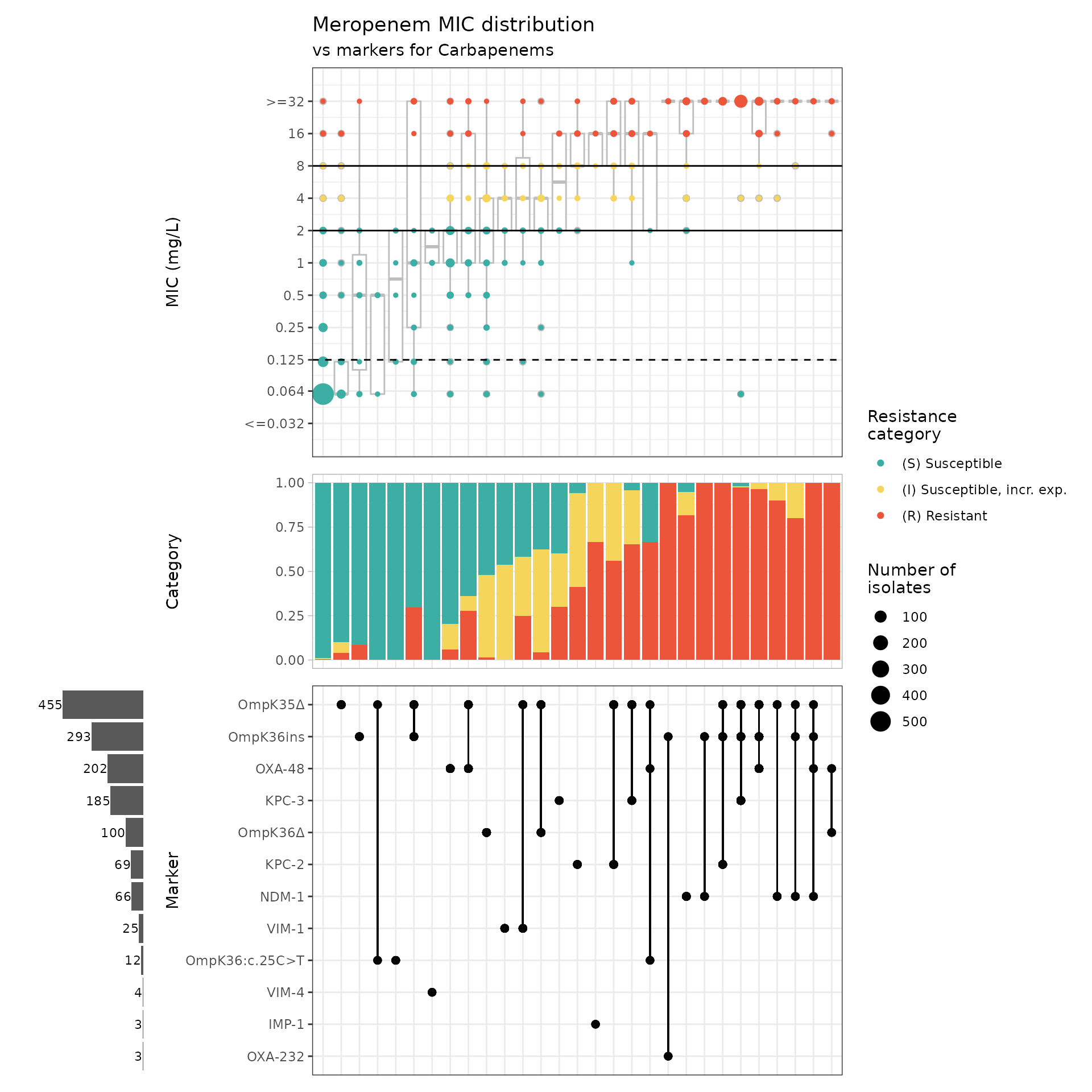
MIC boxplot for Kleborate enzymes vs porin mutations
Now let’s use the assay_by_var() function to explore the
MIC distribution stratified by enzyme, and by mutation. Setting
boxplot=T we can view boxplots of MIC, grouped and coloured
by mutation (setting colour_by="Omp_mutations"), and
faceted to one plotting panel per carbapenemase gene (setting
facet_by = "Bla_Carb_acquired"). This also returns summary
stats (median, interquartile range for MIC) stratified by gene and
mutation. By specifying species="Klebsiella pneumoniae', we
can also retrieve the clinical breakpoints and ECOFF for meropenem and
add these to the plot.
# pivot genotype table to wide format (one row per sample) with separate columns for each class of marker, and add the MIC values for each sample
kleborate_dev_wide_mic <- kleborate_dev_plotting %>%
  filter(marker.label != "OmpK36:c.25C>T") %>% # filter out synonymous SNP
  select(id, Kleborate_Class, marker.label) %>%
  pivot_wider(
    id_cols = id,
    names_from = Kleborate_Class,
    values_from = marker.label,
    values_fn = ~ paste(.x, collapse = ","),
    values_fill = "-"
  ) %>%
  left_join(kp_mero_euscape)
#> Joining with `by = join_by(id)`

head(kleborate_dev_wide_mic)
#> # A tibble: 6 × 61
#>   id          AGly_acquired Fcyn_acquired Flq_acquired Phe_acquired Sul_acquired
#>   <chr>       <chr>         <chr>         <chr>        <chr>        <chr>
#> 1 SAMEA34989… aac(3)-IIa.v… fosA10*?      qnrB4,aac(6… catA1        sul1
#> 2 SAMEA34989… -             fosA5*        -            -            -
#> 3 SAMEA34989… -             fosA10*?      -            catA1        sul2
#> 4 SAMEA34989… aac(3)-IIa.v… fosA10*?      qnrB4,aac(6… catA1        sul1
#> 5 SAMEA34989… aac(3)-IIa.v… fosA5         -            -            -
#> 6 SAMEA34989… -             fosA5         -            -            -
#> # ℹ 55 more variables: Tmt_acquired <chr>, Bla_acquired <chr>,
#> #   Bla_ESBL_acquired <chr>, Bla_chr <chr>, Omp_mutations <chr>,
#> #   Flq_mutations <chr>, MLS_acquired <chr>, Tet_acquired <chr>,
#> #   Col_mutations <chr>, Rif_acquired <chr>, Bla_Carb_acquired <chr>,
#> #   Col_acquired <chr>, Bla_inhR_acquired <chr>, drug <ab>, mic <mic>,
#> #   disk <dsk>, pheno_provided <sir>, pheno_eucast <sir>, ecoff <sir>,
#> #   guideline <chr>, method <chr>, platform <chr>, source <chr>, …

# this table is now ready to use with assay_by_var, to flexibly explore MIC distribution by genotype
kleborate_mic_by_gene_mutation <- assay_by_var(kleborate_dev_wide_mic,
  pheno_drug = "Meropenem", colour_by = "Omp_mutations",
  facet_by = "Bla_Carb_acquired", species = "Klebsiella pneumoniae",
  colour_legend_label = "Porin status", boxplot = T, measure_axis_label = "MIC (mg/L)"
)
#>   MIC breakpoints determined using AMR package: S <= 2 and R > 8
#>   NOTE: Multiple breakpoint entries, for different sites: Non-meningitis; Meningitis. Using the one with the highest S breakpoint (Non-meningitis).

kleborate_mic_by_gene_mutation$plot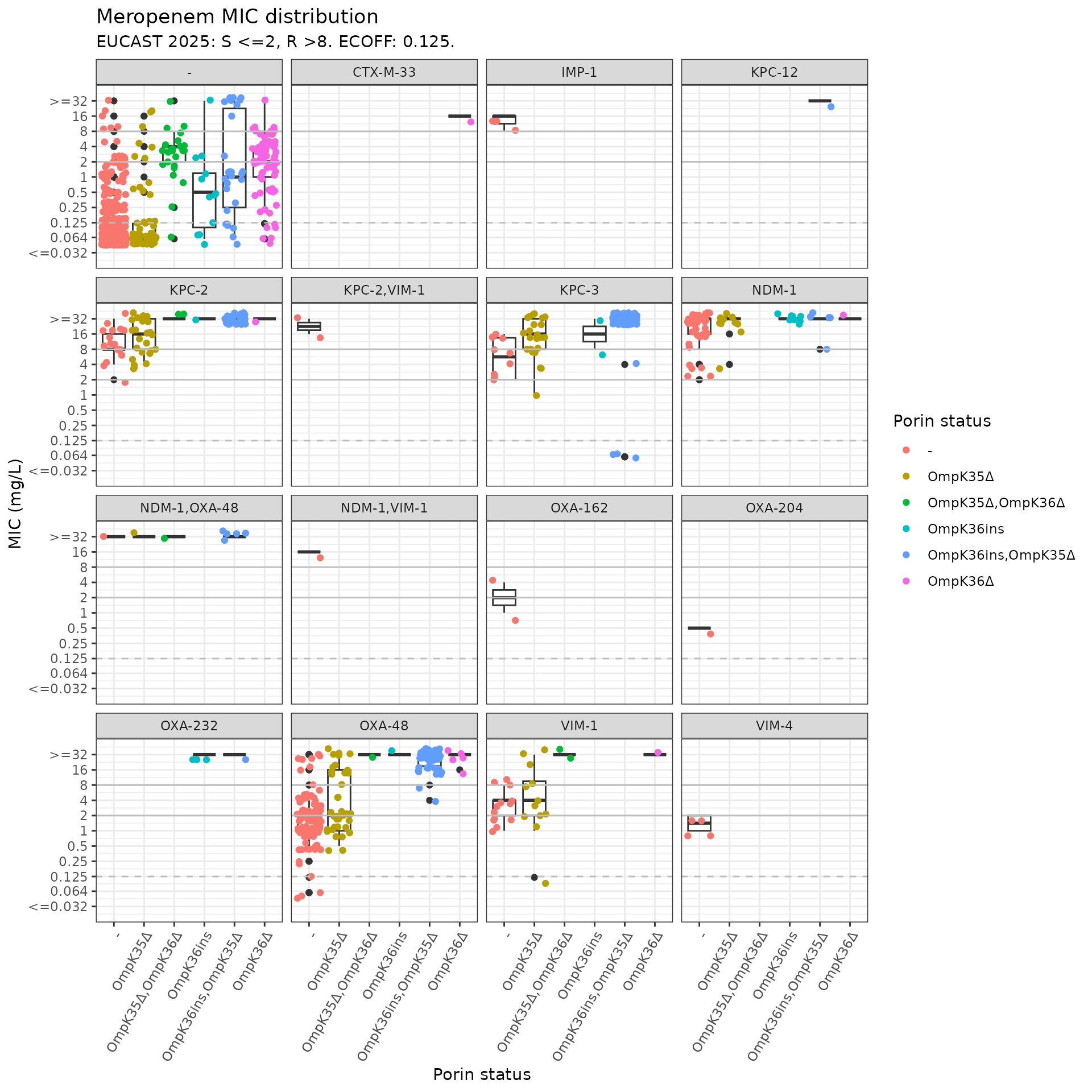
The plot is crowded with some carbapenemase/combinations that are very rare, let’s collapse into enzyme families, exclude isolates that have multiple carbapenemases (n=11), and remove the single CTX gene.
kleborate_dev_wide_mic_trim <- kleborate_dev_wide_mic %>%
  filter(!grepl(",", Bla_Carb_acquired)) %>% # exclude isolates with multiple carbapenemases
  mutate(Bla_Carb_acquired = substr(Bla_Carb_acquired, 1, 3)) %>% # first 3 letters give gene family name
  filter(Bla_Carb_acquired != "CTX")

kleborate_mic_by_gene_mutation <- assay_by_var(kleborate_dev_wide_mic_trim,
  pheno_drug = "Meropenem", colour_by = "Omp_mutations",
  facet_by = "Bla_Carb_acquired", species = "Klebsiella pneumoniae",
  colour_legend_label = "Porin status",
  boxplot = T, measure_axis_label = "MIC (mg/L)"
)
#>   MIC breakpoints determined using AMR package: S <= 2 and R > 8
#>   NOTE: Multiple breakpoint entries, for different sites: Non-meningitis; Meningitis. Using the one with the highest S breakpoint (Non-meningitis).

kleborate_mic_by_gene_mutation$plot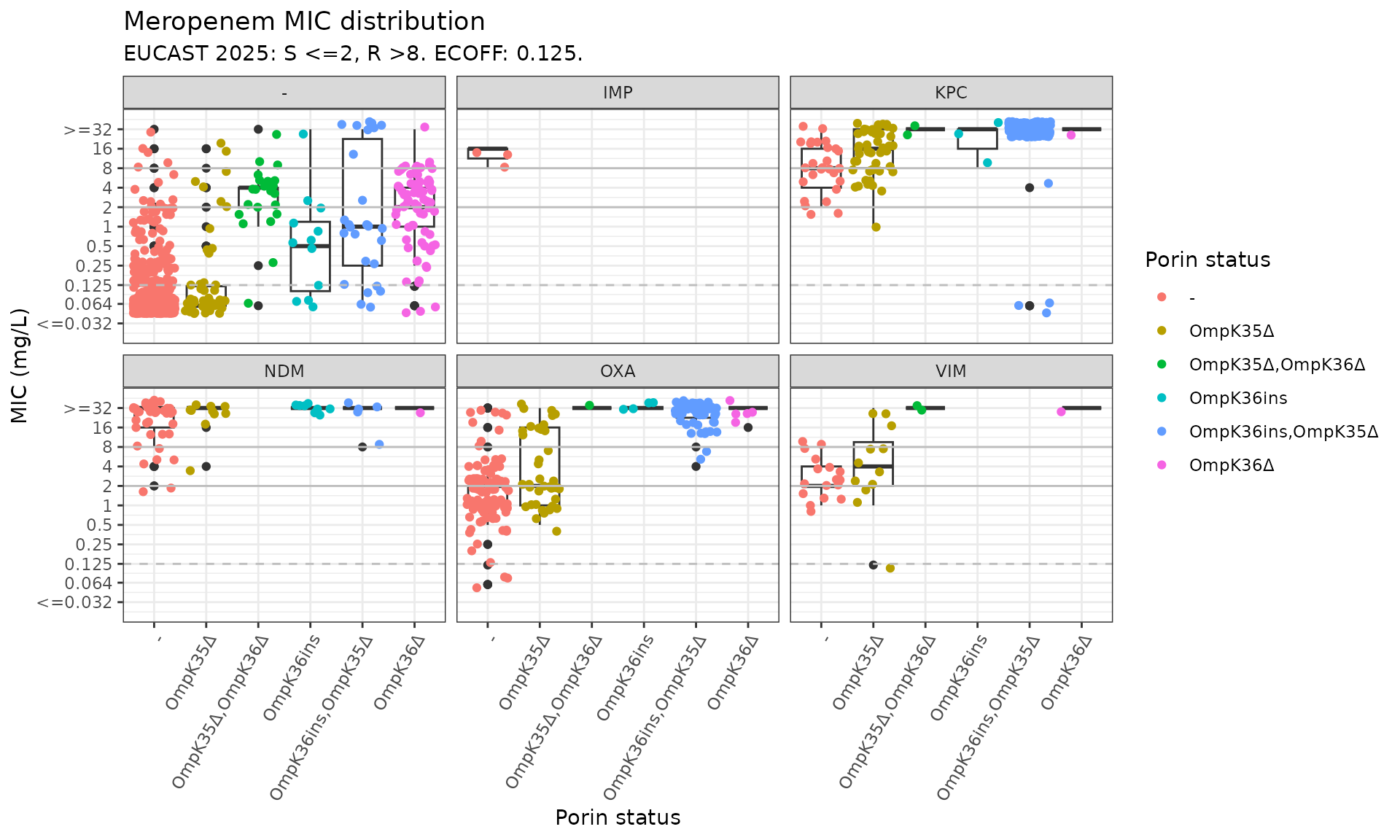
Now we can see the impact of the mutations in the absence of any carbapenemase gene (panel labelled “-”); the MIC distribution associated with each carbapenemase in the absence of any mutation (red points in all other plots); and the impact of mutations in the presence of each type of carbapenemase (other colours).
kleborate_mic_by_gene_mutation$stats %>% head(19)
#> # A tibble: 19 × 7
#>    Omp_mutations   Bla_Carb_acquired     n median geom_mean    q25   q75
#>    <chr>           <chr>             <int>  <dbl>     <dbl>  <dbl> <dbl>
#>  1 -               -                   726   0.06    0.0842  0.06   0.06
#>  2 -               IMP                   3  16      12.7    12     16
#>  3 -               KPC                  27   8       7.80    4     16
#>  4 -               NDM                  38  32      18.9    16     32
#>  5 -               OXA                 103   2       1.56    1      2
#>  6 -               VIM                  17   2       2.55    2      4
#>  7 OmpK35Δ         -                    52   0.06    0.150   0.06   0.12
#>  8 OmpK35Δ         KPC                  48  16      13.3     8     32
#>  9 OmpK35Δ         NDM                  10  32      24.3    32     32
#> 10 OmpK35Δ         OXA                  39   2       3.47    1     16
#> 11 OmpK35Δ         VIM                  12   4       3.99    2     10
#> 12 OmpK35Δ,OmpK36Δ -                    24   4       2.74    2      4
#> 13 OmpK35Δ,OmpK36Δ KPC                   2  32      32      32     32
#> 14 OmpK35Δ,OmpK36Δ OXA                   1  32      32      32     32
#> 15 OmpK35Δ,OmpK36Δ VIM                   2  32      32      32     32
#> 16 OmpK36ins       -                    12   0.5     0.523   0.105  1.25
#> 17 OmpK36ins       KPC                   3  32      20.2    20     32
#> 18 OmpK36ins       NDM                   8  32      32      32     32
#> 19 OmpK36ins       OXA                   4  32      32      32     32
Reformat the stats table into wide format to more clearly see the effects of porin vs. carbapenemase status on MIC. Median and geometric mean (in brackets) values are grouped by porin vs. carbapenemase status, each corresponding to unique boxplotted distribution.
kleborate_mic_by_gene_mutation_table <- kleborate_mic_by_gene_mutation$stats %>%
  mutate(geom_mean = round(geom_mean, 1)) %>%
  mutate(median_mean = paste0(median, " (", geom_mean, ")")) %>%
  mutate(OmpK35 = case_when(
    grepl("OmpK35", Omp_mutations) ~ "\u0394",
    TRUE ~ "-"
  )) %>%
  mutate(OmpK36 = case_when(
    grepl("OmpK36ins", Omp_mutations) ~ "Insertion",
    grepl("OmpK36\u0394", Omp_mutations) ~ "\u0394",
    TRUE ~ "-"
  )) %>%
  mutate(Bla_Carb_acquired = str_replace_all(Bla_Carb_acquired, "-", "None")) %>%
  select(OmpK35, OmpK36, Bla_Carb_acquired, median_mean)

median_MIC_table <- kleborate_mic_by_gene_mutation_table %>%
  pivot_wider(
    names_from = Bla_Carb_acquired,
    values_from = median_mean,
    values_fill = "-"
  )

median_MIC_table
#> # A tibble: 6 × 8
#>   OmpK35 OmpK36    None       IMP       KPC       NDM       OXA       VIM
#>   <chr>  <chr>     <chr>      <chr>     <chr>     <chr>     <chr>     <chr>
#> 1 -      -         0.06 (0.1) 16 (12.7) 8 (7.8)   32 (18.9) 2 (1.6)   2 (2.6)
#> 2 Δ      -         0.06 (0.1) -         16 (13.3) 32 (24.3) 2 (3.5)   4 (4)
#> 3 Δ      Δ         4 (2.7)    -         32 (32)   -         32 (32)   32 (32)
#> 4 -      Insertion 0.5 (0.5)  -         32 (20.2) 32 (32)   32 (32)   -
#> 5 Δ      Insertion 1 (1.5)    -         32 (28.5) 32 (24.3) 32 (25.8) -
#> 6 -      Δ         2 (1.8)    -         32 (32)   32 (32)   32 (27.9) 32 (32)
Making the table aesthetically pleasing using the gt package (to reproduce Figure 5c in the AMRgen paper).
# If you have the gt package, you can use it to make the table aesthetically pleasing
median_MIC_table_aes <- median_MIC_table %>%
gt() %>%
cols_label(
OmpK35 = html("<b>OmpK35</b>"),
OmpK36 = html("<b>OmpK36</b>"),
None = html("<b>None</b>"),
IMP = html("<b>IMP</b>"),
KPC = html("<b>KPC</b>"),
NDM = html("<b>NDM</b>"),
OXA = html("<b>OXA</b>"),
VIM = html("<b>VIM</b>"),
) %>%
tab_spanner(
label = html("<b>Porin status</b>"),
columns = c("OmpK35", "OmpK36")
) %>%
tab_spanner(
label = html("<b>Carbapenemase status</b>"),
columns = c("None", "KPC", "NDM", "OXA", "VIM", "IMP")
) %>%
fmt_missing(
columns = everything(),
missing_text = "-"
) %>%
# Background color based on EUCAST breakpoints
data_color(
columns = c("None", "KPC", "NDM", "OXA", "VIM", "IMP"),
fn = function(x) {
numeric_vals <- as.numeric(str_extract(x, "^[0-9.]+"))
case_when(
is.na(numeric_vals) ~ "transparent",
numeric_vals <= 2 ~ "#3CAEA3",
numeric_vals <= 8 ~ "#F6D55C",
numeric_vals > 8 ~ "#ED553B"
)
}
) %>%
# Changing orange cells to have white font so it is easier to see the numbers
data_color(
columns = c("None", "KPC", "NDM", "OXA", "VIM", "IMP"),
fn = function(x) {
numeric_vals <- as.numeric(str_extract(x, "^[0-9.]+"))
case_when(
is.na(numeric_vals) ~ "black",
numeric_vals > 8 ~ "white",
TRUE ~ "black"
)
},
apply_to = "text"
) %>%
# aligning columns
cols_align(
align = "center",
columns = everything()
) %>%
# text options
tab_options(
table.font.names = "Arial",
table.font.size = 14,
heading.title.font.size = 16,
table.border.top.color = "black",
table.border.bottom.color = "black"
) %>%
# column widths
cols_width(
OmpK35 ~ px(125),
OmpK36 ~ px(125),
everything() ~ px(100)
)
# Adding title and legend for colour
median_MIC_table_aes <- median_MIC_table_aes %>%
tab_header(
title = html("<b>Median (Mean) Meropenem Minimum Inhibitory Concentration (mg/L)</b>"),
subtitle = html(
"<span style='font-size:12px;'>
<b>EUCAST clinical breakpoint:</b>
<span style='color:#3CAEA3;'>■</span> S (Susceptible, ≤ 2 mg/L)
<span style='color:#F6D55C;'>■</span> I (Susceptible, Increased exposure; 4-8 mg/L)
<span style='color:#ED553B;'>■</span> R (Resistant, > 8 mg/L)
</span>"
)
)
median_MIC_table_aesGenotypes from Kleborate v3.1.3
Import Kleborate (<= v3.1.3) Genotype Data
We will now compare the latest version of Kleborate (which we’ve been using up until this point) development branch; commit #4ec1dcb to an older version of Kleborate v3.1.3. The older versions (<=v3.1.3) of Kleborate uses informal nomenclature to describe mutations (e.g. [gene]-[mutation], [gene]-X%, OmpK36GD), whereas the updated version follows the HGVS nomenclature standard.
A table of Kleborate v3.1.3 results generated for the EuSCAPE genomes
is available in the AMRgen package as kleborate_raw_v313.
Let’s import it and summarise its contents:
# View Kleborate output v3.1.3 (using informal nomenclature (e.g. [gene]-[mutation], [gene]-X%, OmpK36GD))
head(kleborate_raw_v313, n = 10)
#> # A tibble: 10 × 113
#>    strain    species species_match contig_count    N50 largest_contig total_size
#>    <chr>     <chr>   <chr>                <dbl>  <dbl>          <dbl>      <dbl>
#>  1 SAMEA349… Klebsi… strong                 141 230759         470757    5578320
#>  2 SAMEA349… Klebsi… strong                  88 370309         938079    5384685
#>  3 SAMEA349… Klebsi… strong                  90 238750         529125    5446454
#>  4 SAMEA349… Klebsi… strong                 144 207582         663698    5574298
#>  5 SAMEA349… Klebsi… strong                 142 263498         678692    5486238
#>  6 SAMEA349… Klebsi… strong                  79 285199         991412    5529803
#>  7 SAMEA349… Klebsi… strong                 280 178980         585359    5817055
#>  8 SAMEA349… Klebsi… strong                 108 209418         517450    5379124
#>  9 SAMEA349… Klebsi… strong                 134 371444         984005    5558705
#> 10 SAMEA349… Klebsi… strong                 142 197944         636773    5497421
#> # ℹ 106 more variables: ambiguous_bases <chr>, QC_warnings <chr>, ST <chr>,
#> #   gapA <dbl>, infB <dbl>, mdh <dbl>, pgi <dbl>, phoE <dbl>, rpoB <dbl>,
#> #   tonB <dbl>, YbST <chr>, Yersiniabactin <chr>, ybtS <chr>, ybtX <chr>,
#> #   ybtQ <chr>, ybtP <chr>, ybtA <chr>, irp2 <chr>, irp1 <chr>, ybtU <chr>,
#> #   ybtT <chr>, ybtE <chr>, fyuA <chr>, spurious_ybt_hits <chr>, CbST <chr>,
#> #   Colibactin <chr>, clbA <chr>, clbB <chr>, clbC <chr>, clbD <chr>,
#> #   clbE <chr>, clbF <chr>, clbG <chr>, clbH <chr>, clbI <chr>, clbL <chr>, …

# Use import_kleborate() function and set `hgvs = FALSE` for Kleborate outputs generated from <=v3.1.3 (using non-HGVS nomenclature)
kleborate_v313 <- import_kleborate(
  input_table = kleborate_raw_v313,
  sample_col = "strain",
  hgvs = FALSE
)

# Summarize genotype table
summarise_geno(kleborate_v313, sample_col = "id", marker_col = "marker.label")
#> $uniques
#> # A tibble: 6 × 2
#>   column         n_unique
#>   <chr>             <int>
#> 1 id                 1489
#> 2 marker.label        263
#> 3 drug                  1
#> 4 drug_class           13
#> 5 gene                263
#> 6 variation type        4
#>
#> $per_type
#> # A tibble: 4 × 6
#>   `variation type`                  id marker.label  drug drug_class  gene
#>   <chr>                          <int>        <int> <int>      <int> <int>
#> 1 Gene presence detected          1489          246     1         13   246
#> 2 Inactivating mutation detected   568            3     1          2     3
#> 3 Nucleotide variant detected       15            1     1          1     1
#> 4 Protein variant detected         874           13     1          2    13
#>
#> $drugs
#> # A tibble: 13 × 5
#>    drug  drug_class                markers samples  hits
#>    <lgl> <chr>                       <int>   <int> <int>
#>  1 NA    Aminoglycosides                59    1057  3140
#>  2 NA    Beta-lactams                   76    1457  2833
#>  3 NA    Carbapenems                    17     766  1459
#>  4 NA    Cephalosporins (3rd gen.)      18     648   668
#>  5 NA    Macrolides                     14     460   923
#>  6 NA    Phenicols                      12     469   558
#>  7 NA    Phosphonics                     1       3     3
#>  8 NA    Polymyxins                      3     138   138
#>  9 NA    Quinolones                     25    1020  2422
#> 10 NA    Rifamycins                      2     114   114
#> 11 NA    Sulfonamides                    9     913  1090
#> 12 NA    Tetracyclines                   9     503   541
#> 13 NA    Trimethoprims                  18     886  1017
#>
#> $markers
#> # A tibble: 263 × 5
#>    marker.label drug  drug_class                `variation type`           n
#>    <chr>        <lgl> <chr>                     <chr>                  <int>
#>  1 ACC-4        NA    Beta-lactams              Gene presence detected     2
#>  2 CMY-13       NA    Beta-lactams              Gene presence detected     1
#>  3 CMY-16       NA    Beta-lactams              Gene presence detected    31
#>  4 CMY-2.v2     NA    Beta-lactams              Gene presence detected     1
#>  5 CMY-30       NA    Cephalosporins (3rd gen.) Gene presence detected     1
#>  6 CMY-4.v1     NA    Beta-lactams              Gene presence detected     5
#>  7 CMY-6        NA    Beta-lactams              Gene presence detected     2
#>  8 CTX-M-1      NA    Cephalosporins (3rd gen.) Gene presence detected     1
#>  9 CTX-M-14     NA    Cephalosporins (3rd gen.) Gene presence detected    16
#> 10 CTX-M-15     NA    Cephalosporins (3rd gen.) Gene presence detected   568
#> # ℹ 253 more rows
Compare Kleborate versions
Comparing only the carbapenem resistance determinants from an updated version Kleborate (development branch) to a previous version (v3.1.3).
# Grouping Kleborate development branch carbapenem resistance determinants, so that there is one row per sample
kleborate_dev_markers_grouped <- kleborate_dev %>%
  filter(Kleborate_Class == "Omp_mutations" | Kleborate_Class == "Bla_Carb_acquired") %>%
  select(id, marker.label) %>%
  rename(kleborate = marker.label) %>%
  group_by(id) %>%
  summarise(
    Kleborate_dev_markers = kleborate %>%
      sort() %>%
      str_c(collapse = ";")
  )

# Since we know that Kleborate v3.1.3 does not use HGVS notation, we will change the names of the OmpK36 mutations to match HGVS notation for comparison purposes
# After, we group them so there is one row per sample
kleborate_v313_markers_grouped <- kleborate_v313 %>%
  filter(Kleborate_Class == "Omp_mutations" | Kleborate_Class == "Bla_Carb_acquired") %>%
  select(id, marker.label) %>%
  mutate(
    marker.label = str_replace_all(marker.label, "OmpK36GD", "OmpK36:p.134_135insGD"),
    marker.label = str_replace_all(marker.label, "OmpK36_c25t", "OmpK36:c.25C>T"),
    marker.label = str_replace_all(marker.label, "OmpK36TD", "OmpK36:p.136_137insTD")
  ) %>%
  rename(kleborate = marker.label) %>%
  group_by(id) %>%
  summarise(
    Kleborate_v313_markers = kleborate %>%
      sort() %>%
      str_c(collapse = ";")
  )

# Joining Kleborate version tables for comparison
compare_kleborate_versions <- full_join(
  kleborate_dev_markers_grouped,
  kleborate_v313_markers_grouped
)
#> Joining with `by = join_by(id)`

# Comparing Kleborate versions and creating two new columns to show what each version is missing
compare_kleborate_versions <- compare_kleborate_versions %>%
  rowwise() %>%
  mutate(
    dev_missing = {
      v313_vec <- str_split(Kleborate_v313_markers, ";")[[1]]
      dev_vec <- str_split(Kleborate_dev_markers, ";")[[1]]
      missing <- setdiff(v313_vec, dev_vec)
      if (length(missing) == 0) NA_character_ else str_c(missing, collapse = ";")
    },
    v313_missing = {
      v313_vec <- str_split(Kleborate_v313_markers, ";")[[1]]
      dev_vec <- str_split(Kleborate_dev_markers, ";")[[1]]
      missing <- setdiff(dev_vec, v313_vec)
      if (length(missing) == 0) NA_character_ else str_c(missing, collapse = ";")
    }
  ) %>%
  ungroup()

# Table listing the AMR markers that are missing from Kleborate v3.1.3
compare_kleborate_versions %>% count(v313_missing, sort = TRUE)
#> # A tibble: 4 × 2
#>   v313_missing             n
#>   <chr>                <int>
#> 1 NA                     752
#> 2 OmpK36:p.135_136insD    12
#> 3 OmpK35:-                 4
#> 4 OmpK36:-                 2

# Table listing the AMR markers that are missing from the updated Kleborate version
compare_kleborate_versions %>% count(dev_missing, sort = TRUE)
#> # A tibble: 1 × 2
#>   dev_missing     n
#>   <chr>       <int>
#> 1 NA            770
We can see that there are no carbapenem resistance determinants missed by the updated Kleborate development version, in fact, the new version now additionally calls OmpK36:p.135_136insD (n=12), and OmpK35:- (n=4), and OmpK36:- (n=2) that were previously unidentified.
Noting that there are no new carbapenem resistance genes identified in this new version of Kleborate which includes an updated AMR database.
Up until this point, we have only explored using different versions of Kleborate as the AMR genotyper. The next few sections will explore using different AMR genotypers and comparing their results.
First up, we have AMRFinderPlus!
Genotypes from AMRFinderPlus
NCBI has developed AMRFinderPlus, a tool that identifies AMR genes, resistance-associated point mutations, and select other classes of genes using protein annotations and/or assembled nucleotide sequence, published here. It can only be used via command line and also has organism-specific options.
Import AMRFinderPlus Genotype Data
The download_ebi() can download AMRFinderPlus genotype data from the EBI AMR portal, filter your species of interest, and reformat into AMRgen genotype table. The AMRFinderPlus data being used here is from the 2025-12 release using AMRFinderPlus version v4.0. Noting that as of AMRFinderPlus (v4.2.5), there is additional functionality to identify putatively function disrupting mutations in genes (i.e., ompk35 and ompk36 loss and truncations) that lead to resistance, which Kleborate already identifies.
# Download Klebsiella pneumoniae genotype AMRFinderPlus data and re-format the data into an AMRgen genotype table
amrfp <- download_ebi(
  data = "genotype", species = "Klebsiella pneumoniae",
  reformat = T
)

# Filter for isolates in EuSCAPE paper with meropenem phenotypes and remove contaminated samples
kp_mero_amrfp <- kp_mero_amrfp %>%
  filter(id %in% kp_mero_euscape$id) %>%
  filter(!id %in% contaminated_assemblies)
A copy of this data frame is avaiable in the AMRgen pacakge as
kp_mero_amrfp:
head(kp_mero_amrfp)
#> # A tibble: 6 × 34
#>   id        marker gene  mutation drug_agent drug_class marker.label assembly_ID
#>   <chr>     <chr>  <chr> <chr>    <ab>       <chr>      <chr>        <chr>
#> 1 SAMEA364… ompK3… ompK… Asp135A… NA         Carbapene… ompK36:Asp1… GCA_900500…
#> 2 SAMEA364… gyrA_… gyrA  Ser83Ile NA         Quinolones gyrA:Ser83I… GCA_900500…
#> 3 SAMEA364… fosA   fosA  -        FOS        Phosphoni… fosA         GCA_900500…
#> 4 SAMEA364… parC_… parC  Ser80Ile NA         Quinolones parC:Ser80I… GCA_900500…
#> 5 SAMEA364… oqxB   oqxB  -        NA         Phenicols  oqxB         GCA_900500…
#> 6 SAMEA364… oqxB   oqxB  -        NA         Quinolones oqxB         GCA_900500…
#> # ℹ 26 more variables: genus <chr>, species <chr>, organism <chr>,
#> #   isolate <chr>, taxon_id <int>, region <chr>, region_start <int>,
#> #   region_end <int>, strand <chr>, `_bin` <int>, id2 <chr>, gene_symbol <chr>,
#> #   amr_element_symbol <chr>, element_type <chr>, element_subtype <chr>,
#> #   class <chr>, subclass <chr>, split_subclass <chr>, antibiotic_name <chr>,
#> #   antibiotic_ontology <chr>, antibiotic_ontology_link <chr>,
#> #   evidence_accession <chr>, evidence_type <chr>, evidence_link <chr>, …

# Summary of carbapenem resistance determinants
summarise_geno(kp_mero_amrfp)
#> $uniques
#> # A tibble: 4 × 2
#>   column     n_unique
#>   <chr>         <int>
#> 1 id             1490
#> 2 marker          237
#> 3 drug_class       20
#> 4 gene            218
#>
#> $per_type
#> NULL
#>
#> $drugs
#> # A tibble: 20 × 4
#>    drug_class                markers samples     n
#>    <chr>                       <int>   <int> <int>
#>  1 Aminoglycosides                35    1020  6046
#>  2 Beta-lactams                   45    1424  2353
#>  3 Carbapenems                    16     669   956
#>  4 Cephalosporins                  1      23    48
#>  5 Cephalosporins (3rd gen.)      36     788  1479
#>  6 Efflux                          1    1483  1483
#>  7 Glycopeptides                   1      49    49
#>  8 Lincosamides                    3       3     5
#>  9 Macrolides                      7     479  6818
#> 10 Other                           1       2     4
#> 11 Penicillins                     1       4    16
#> 12 Phenicols                      25    1458  3802
#> 13 Phosphonics                     5    1488  1491
#> 14 Polymyxins                     12      40    40
#> 15 Quinolones                     40    1468  4959
#> 16 Rifamycins                      3     110   119
#> 17 Streptogramins                  2      83   249
#> 18 Sulfonamides                    3     931  1206
#> 19 Tetracyclines                  12     605   699
#> 20 Trimethoprims                  12     539   563
#>
#> $markers
#> # A tibble: 261 × 3
#>    marker        drug_class          n
#>    <chr>         <chr>           <int>
#>  1 aac(3)-IId    Aminoglycosides   122
#>  2 aac(3)-IIe    Aminoglycosides   379
#>  3 aac(3)-IIg    Aminoglycosides    14
#>  4 aac(3)-IVa    Aminoglycosides    45
#>  5 aac(3)-Ia     Aminoglycosides     5
#>  6 aac(3)-VIa    Aminoglycosides     1
#>  7 aac(6')-IIc   Aminoglycosides   189
#>  8 aac(6')-Ib    Aminoglycosides  3100
#>  9 aac(6')-Ib'   Aminoglycosides    11
#> 10 aac(6')-Ib-cr Aminoglycosides    24
#> # ℹ 251 more rows
Compare AMRFinderPlus to Kleborate genotype results
We are going to compare the AMRFinderPlus results that we just downloaded and the Kleborate development branch results. We know that there are differences between AMRFinderPlus and Kleborate development branch in detecting porin defects:
Kleborate development branch does not identify OmpK35_E132K. As per NCBI Reference Gene Catalog, the citation related to this mutation is PMID: 20660684. In the paper, the mutation (ompK35_E132K) is detected in a strain (AIS080884) with an ompk36 mutation (Ser255Thr) that is categorized as low carbapenem resistance. There is no other other literature that experimentally tests this mutation alone, other papers only report the presence of the mutation (often in combination with other mutations/carbapenemases).
AMRFinderPlus (<v4.2.5) only does not detect nucleotide mutations (e.g., OmpK36_c25t), nor does it detect loss of OmpK35/36 (e.g., OmpK35:- or OmpK36:-).
As such, these differences make it difficult to compare, so we will
simplify and remove OmpK35:- and OmpK36:- from
the Kleborate development branch results.
# To count and see the names of the carbapenem resistance determinants
kp_mero_amrfp %>%
  filter(drug_class == "Carbapenems") %>%
  count(marker, sort = TRUE)
#> # A tibble: 16 × 2
#>    marker             n
#>    <chr>          <int>
#>  1 ompK36_D135DGD   281
#>  2 blaOXA-48        219
#>  3 blaKPC-3         194
#>  4 blaKPC-2          77
#>  5 blaNDM-1          73
#>  6 blaVIM-1          32
#>  7 blaVIM-4          25
#>  8 ompK35_E132K      22
#>  9 ompK36_D135DD     12
#> 10 ompK36_T136TDT     9
#> 11 blaOXA-232         4
#> 12 blaIMP-1           3
#> 13 blaOXA-162         2
#> 14 blaNDM             1
#> 15 blaOXA-204         1
#> 16 blaOXA-427         1

# Massaging AMRfp marker names to match Kleborate names
amrfp_simplified <- kp_mero_amrfp %>%
  filter(drug_class == "Carbapenems") %>%
  mutate(
    marker_amrfp = str_replace_all(marker, "bla", ""),
    marker_amrfp = str_replace_all(marker_amrfp, "ompK36_D135DGD", "OmpK36:p.134_135insGD"),
    marker_amrfp = str_replace_all(marker_amrfp, "ompK36_D135DD", "OmpK36:p.135_136insD"),
    marker_amrfp = str_replace_all(marker_amrfp, "ompK36_T136TDT", "OmpK36:p.136_137insTD")
  ) %>%
  select(id, marker_amrfp) %>%
  rename(AMRfp = marker_amrfp) %>%
  group_by(id) %>%
  summarise(
    AMRfp_markers = AMRfp %>%
      sort() %>%
      str_c(collapse = ";")
  )

# Filtering Kleborate AMR markers
# Excluding `OmpK35:-` and `OmpK36:-` since we know that AMRfinderplus (<v4.2.5) does not detect loss/truncations of OmpK35 and OmpK36
kleborate_dev_simplified <- kleborate_dev %>%
  filter(Kleborate_Class == "Omp_mutations" | Kleborate_Class == "Bla_Carb_acquired") %>%
  select(id, marker.label) %>%
  rename(kleborate = marker.label) %>%
  filter(!kleborate %in% c("OmpK35:-", "OmpK36:-")) %>%
  group_by(id) %>%
  summarise(
    Kleborate_markers = kleborate %>%
      sort() %>%
      str_c(collapse = ";")
  )

# Joining AMRFinderPlus and Kleborate tables
compare_amrfp_kleborate <- full_join(
  amrfp_simplified,
  kleborate_dev_simplified
)
#> Joining with `by = join_by(id)`

# Comparing AMRFinderPlus and Kleborate tables and creating two new columns to show what AMRFinderPlus is missing and what Kleborate is missing
compare_amrfp_kleborate <- compare_amrfp_kleborate %>%
  rowwise() %>%
  mutate(
    Kleborate_dev_missing = {
      amr_vec <- str_split(AMRfp_markers, ";")[[1]]
      kleb_vec <- str_split(Kleborate_markers, ";")[[1]]
      missing <- setdiff(amr_vec, kleb_vec)
      if (length(missing) == 0) NA_character_ else str_c(missing, collapse = ";")
    },
    AMRfp_missing = {
      amr_vec <- str_split(AMRfp_markers, ";")[[1]]
      kleb_vec <- str_split(Kleborate_markers, ";")[[1]]
      missing <- setdiff(kleb_vec, amr_vec)
      if (length(missing) == 0) NA_character_ else str_c(missing, collapse = ";")
    }
  ) %>%
  ungroup()

# Table listing the AMR markers that are missing from Kleborate (but detected in AMRFinderPlus)
compare_amrfp_kleborate %>% count(Kleborate_dev_missing, sort = TRUE)
#> # A tibble: 11 × 2
#>    Kleborate_dev_missing     n
#>    <chr>                 <int>
#>  1 NA                      610
#>  2 ompK35_E132K             22
#>  3 VIM-4                    21
#>  4 OXA-48                   10
#>  5 KPC-3                     7
#>  6 OmpK36:p.134_135insGD     3
#>  7 KPC-2                     2
#>  8 NDM-1                     2
#>  9 NDM                       1
#> 10 OXA-427                   1
#> 11 VIM-1                     1

# Table listing the AMR markers that are missing from AMRFinderPlus (but detected in Kleborate)
compare_amrfp_kleborate %>% count(AMRfp_missing, sort = TRUE)
#> # A tibble: 4 × 2
#>   AMRfp_missing      n
#>   <chr>          <int>
#> 1 NA               663
#> 2 OmpK36:c.25C>T    15
#> 3 CTX-M-33           1
#> 4 KPC-12             1
Since we know there are differences in porin defect detection between
Kleborate and AMRFinderPlus, we can focus on the carbapenemase
detection. AMRFinderPlus is missing the detection of
CTX-M-33 in one genome and KPC-12 in another
genome.
CTX-M-33
However, AMRFinderPlus is not “missing” CTX-M-33 and
KPC-12 in their database. In the case of
CTX-M-33, it is detected in n=1 genome and is annotated as
conferring resistance to Cephalosporins (3rd gen.) instead
of Carbapenems, which is why it has been excluded from the
AMR genotype table since we filtered for
drug_class=="Carbapenems".
# CTX-M-33 is annotated as conferring resistance to Cephalosporins (3rd gen.) and is identified by AMRFinderPlus in Sample SAMEA3721133
kp_mero_amrfp %>%
  filter(gene == "blaCTX-M-33") %>%
  select(id, gene, drug_class)
#> # A tibble: 1 × 3
#>   id           gene        drug_class
#>   <chr>        <chr>       <chr>
#> 1 SAMEA3721133 blaCTX-M-33 Cephalosporins (3rd gen.)

# Confirming that CTX-M-33 is identified in SAMEA3721133 using Kleborate development branch
compare_amrfp_kleborate %>%
  filter(AMRfp_missing == "CTX-M-33") %>%
  select(id, AMRfp_markers, Kleborate_markers)
#> # A tibble: 1 × 3
#>   id           AMRfp_markers Kleborate_markers
#>   <chr>        <chr>         <chr>
#> 1 SAMEA3721133 NA            CTX-M-33

# Checking phenotype of SAMEA3721133
kp_mero_euscape %>%
  filter(id == "SAMEA3721133") %>%
  select(id, mic, pheno_eucast, ecoff)
#> # A tibble: 1 × 4
#>   id             mic pheno_eucast ecoff
#>   <chr>        <mic> <sir>        <sir>
#> 1 SAMEA3721133    16   R           NWT
The primary literature that describes CTX-M-33 by Galani, et
al. describes the clinical strain of E. coli 2439
harbouring CTX-M-33, E. coli RC85 recipient, and E.
coli 2439 transconjugant (aka E. coli RC85 recipient + CTX-M-33).
The authors performed antibiotic susceptibility tests on E.
coli RC85 recipient and E. coli 2439 transconjugant which
showed that MIC for third gen cephalosporins increased, but the MIC for
imipenem remained the when harbouring CTX-M-33. In the Comprehensive
Antibiotic Resistance Database (CARD, v4.0.1) CTX-M-33 is annotated
as conferring resistance to cephalosporins (not carbapenems). The
EuSCAPE isolate (SAMEA3721133 from above) only harbours CTM-M-33 and is
meropenem resistant. Based on this conflicting evidence, it is unclear
if CTX-M-33 in K. pneumoniae confers resistance to
carbapenems. The experimental work was performed in an E. coli
strain and not K. pneumoniae and only imipenem was the only
carbapenem tested. Additional experimental work and epidemiological
support from K. pneumoniae strains harbouring CTX-M-33 with
carbapenem susceptibility test results is needed to understand the
substrate activity of CTX-M-33.
KPC-12
Similarly, in the case of KPC-12, it is detected in n=1
genome using AMRFinderPlus and is annotated as conferring resistance to
Cephalosporins (3rd gen.) instead of
Carbapenems, which is why it has been excluded from the
genotype table since we filtered for
drug_class=="Carbapenems".
# KPC-12 is annotated as conferring resistance to Cephalosporins (3rd gen.)  and is identified by AMRFinderPlus in Sample SAMEA3649729
kp_mero_amrfp %>%
  filter(gene == "blaKPC-12") %>%
  select(id, gene, drug_class)
#> # A tibble: 1 × 3
#>   id           gene      drug_class
#>   <chr>        <chr>     <chr>
#> 1 SAMEA3649729 blaKPC-12 Cephalosporins (3rd gen.)

# Confirming that KPC-12 is identified in SAMEA3649729 using Kleborate. It also harbours OmpK36:p.134_135insGD
compare_amrfp_kleborate %>%
  filter(AMRfp_missing == "KPC-12") %>%
  select(id, AMRfp_markers, Kleborate_markers)
#> # A tibble: 1 × 3
#>   id           AMRfp_markers         Kleborate_markers
#>   <chr>        <chr>                 <chr>
#> 1 SAMEA3649729 OmpK36:p.134_135insGD KPC-12;OmpK36:p.134_135insGD

# Checking phenotype of SAMEA3649729
kp_mero_euscape %>%
  filter(id == "SAMEA3649729") %>%
  select(id, mic, pheno_eucast, ecoff)
#> # A tibble: 1 × 4
#>   id             mic pheno_eucast ecoff
#>   <chr>        <mic> <sir>        <sir>
#> 1 SAMEA3649729    32   R           NWT
The only primary literature discussing KPC-12 is by Han, et al. where they
show that a strain of E. coli DH5alpha + empty plasmid
vs. E. coli DH5alpha + plasmid with KPC-12 does
not change meropenem MIC (0.06mg/L) with small elevation in imipenem
(0.25 vs. 1 mg/L) and ertapenem (<=0.12mg/L vs. 0.25 mg/L) MICs.
Whereas, E. coli DH5alpha + empty plasmid vs. E. coli
DH5alpha + plasmid with KPC-12 elevates the MICs for
ceftriaxone (<=0.25 vs. >=64 mg/L, 3rd gen cephalosporin) and
cefuroxime (8 vs. 256 mg/L, 2nd gen cephalosporin). This experiment was
performed in an E. coli strain, not K. pneumoniae. In
the EuSCAPE dataset (from above), there is only one isolate
(SAMEA3649729) with KPC-12, which harbours both KPC-12 and
OmpK36:p.134_135insGD and is meropenem resistant. Based on this
conflicting evidence, it is not clear whether KPC-12 should
be changed to conferring resistance to 3rd generation cephalosporins or
carbapenems. Similar to Kleborate, CARD v4.0.1 also has KPC-12 annotated as a
carbapenemase. Further experimental work performed in a K.
pneumoniae strain and having additional evidence from K.
pneumoniae strains with genotype-phenotype data can help strengthen
our understanding of its substrate specificity.
We will not continue to investigate what is missing in the Kleborate development branch, compared to AMRFinderPlus, for the purpose and lengthiness of this vignette. These two examples act as ways to investigate differences in AMR genotypers and how ultimately, choosing a specific genotyper will impact the foundation upon which we understand AMR genotype-phenotype relationships.
Next up, we have the Resistance Gene Identifier (RGI)!
Genotypes from Resistance Gene Identifier (RGI)
RGI identifies resistance determinants from protein or nucleotide data using homology and mutation models, published here. The software uses reference data from the Comprehensive Antibiotic Resistance Database. It can be run via the website or on the command line.
CARD is an ontology-drive database including resistance genes, their
products, and the antibiotics they confer resistance towards. CARD
operates at both a drug class and drug-specific level, where curators
can establish gene confers_resistance_to_drug antibiotic
relationships. Lastly, CARD includes both intrinsic/core and acquired
resistance determinants.
Import Resistance Gene Identifier (RGI) results
Import RGI results using the import_rgi() function. This
function imports and processes genotyping results from RGI extracting
antimicrobial resistance determinants and mapping them to standardised
drug classes/antibiotics. It also shortens determinant names using
CARD Short Names as provided by CARD (https://card.mcmaster.ca/download in
aro_index.tsv).
Note: Check the number of genomes that you expect
using summarise_geno(). RGI text output will be empty if
there are no AMR determinants identified in the submitted genome, so you
have to either:
Add sample IDs with no AMR determinants into the
ORF_IDcolumn of the RGI text output that you are importing, orList your sample IDs in a vector using the
samples_no_amr=parameter in theimport_rgi()function. For example,import_rgi(rgi_EuSCAPE_raw, samples_no_amr = c("SampleA_noAMR", "SampleB_noAMR", "SampleC_noAMR"))
The data frame rgi_EuSCAPE_raw included in the AMRgen
package provides CARD RGI calls for the EuSCAPE genomes:
# Sample IDs with no AMR determinants have been added to rgi_EuSCAPE_raw under the `ORF_ID` column with the rest of the rows left blank
tail(rgi_EuSCAPE_raw, n = 10)
#> # A tibble: 10 × 26
#>    ORF_ID Contig Start  Stop Orientation Cut_Off Pass_Bitscore Best_Hit_Bitscore
#>    <chr>   <dbl> <dbl> <dbl> <chr>       <chr>           <dbl>             <dbl>
#>  1 SAMEA…     NA    NA    NA NA          NA                 NA                NA
#>  2 SAMEA…     NA    NA    NA NA          NA                 NA                NA
#>  3 SAMEA…     NA    NA    NA NA          NA                 NA                NA
#>  4 SAMEA…     NA    NA    NA NA          NA                 NA                NA
#>  5 SAMEA…     NA    NA    NA NA          NA                 NA                NA
#>  6 SAMEA…     NA    NA    NA NA          NA                 NA                NA
#>  7 SAMEA…     NA    NA    NA NA          NA                 NA                NA
#>  8 SAMEA…     NA    NA    NA NA          NA                 NA                NA
#>  9 SAMEA…     NA    NA    NA NA          NA                 NA                NA
#> 10 SAMEA…     NA    NA    NA NA          NA                 NA                NA
#> # ℹ 18 more variables: Best_Hit_ARO <chr>, Best_Identities <dbl>, ARO <dbl>,
#> #   Model_type <chr>, SNPs_in_Best_Hit_ARO <chr>, Other_SNPs <chr>,
#> #   `Drug Class` <chr>, `Resistance Mechanism` <chr>, `AMR Gene Family` <chr>,
#> #   `Percentage Length of Reference Sequence` <dbl>, ID <chr>, Model_ID <dbl>,
#> #   Nudged <lgl>, Note <lgl>, Hit_Start <dbl>, Hit_End <dbl>, Antibiotic <chr>,
#> #   AST_Source <chr>

# Import RGI output with n=1490 isolates
rgi <- import_rgi(rgi_EuSCAPE_raw)

# Summarize genotype data
summarise_geno(rgi)
#> $uniques
#> # A tibble: 5 × 2
#>   column         n_unique
#>   <chr>             <int>
#> 1 id                 1490
#> 2 marker              252
#> 3 drug                109
#> 4 drug_class           30
#> 5 variation type        3
#>
#> $per_type
#> # A tibble: 3 × 5
#>   `variation type`            id marker  drug drug_class
#>   <chr>                    <int>  <int> <int>      <int>
#> 1 Gene presence detected    1430    233    98         29
#> 2 Protein variant detected  1445     18    37         13
#> 3 NA                          45      1     1          1
#>
#> $drugs
#> # A tibble: 114 × 5
#>    drug                 drug_class       markers samples  hits
#>    <chr>                <chr>              <int>   <int> <int>
#>  1 2'-N-ethylnetilmicin Aminoglycosides        8     462   492
#>  2 5-episisomicin       Aminoglycosides        3      37    37
#>  3 6'-N-ethylnetilmicin Aminoglycosides        6     449   456
#>  4 AMK                  Aminoglycosides       18    1445  3846
#>  5 AMP                  Aminopenicillins      22    1445 10675
#>  6 AMX                  Aminopenicillins       6     747  1110
#>  7 APR                  Aminoglycosides        1       5     5
#>  8 ARB                  Aminoglycosides        4      72    73
#>  9 AST                  Aminoglycosides        2      17    17
#> 10 ATM                  Monobactams            1       1     1
#> # ℹ 104 more rows
#>
#> $markers
#> # A tibble: 815 × 5
#>    marker     drug                 drug_class      `variation type`           n
#>    <chr>      <chr>                <chr>           <chr>                  <int>
#>  1 AAC(3)-IIc 2'-N-ethylnetilmicin Aminoglycosides Gene presence detected    16
#>  2 AAC(3)-IIc 6'-N-ethylnetilmicin Aminoglycosides Gene presence detected    16
#>  3 AAC(3)-IIc DKB                  Aminoglycosides Gene presence detected    16
#>  4 AAC(3)-IIc GEN                  Aminoglycosides Gene presence detected    16
#>  5 AAC(3)-IIc NET                  Aminoglycosides Gene presence detected    16
#>  6 AAC(3)-IIc SIS                  Aminoglycosides Gene presence detected    16
#>  7 AAC(3)-IIc TOB                  Aminoglycosides Gene presence detected    16
#>  8 AAC(3)-IId 2'-N-ethylnetilmicin Aminoglycosides Gene presence detected    88
#>  9 AAC(3)-IId 6'-N-ethylnetilmicin Aminoglycosides Gene presence detected    88
#> 10 AAC(3)-IId DKB                  Aminoglycosides Gene presence detected    88
#> # ℹ 805 more rows
Generate Binary Matrix for RGI AMR Markers
rgi_binary_matrix <- get_binary_matrix(
  geno_table = rgi,
  pheno_table = kp_mero_euscape,
  pheno_drug = "Meropenem",
  geno_class = c("Carbapenems"),
  sir_col = "pheno_eucast",
  marker_col = "marker.label",
  keep_assay_values = TRUE,
  keep_assay_values_from = "mic"
)
#>  Defining NWT in binary matrix using ecoff column provided: ecoff
Solo PPV Analysis for RGI AMR Markers
# No solo markers error when you run solo_ppv()! Since CARD/RGI includes intrinsic and acquired resistance determinants, there could be intrinsic / core resistance determinants that are found across most (if not all) genomes which obstructs our view of carbapenem resistance determinants found alone.

soloPPV_rgi_mero <- solo_ppv(binary_matrix = rgi_binary_matrix)
As such, we will exclude the core/intrinsic resistance determinants, using their prevalence and exclude any determinants identified across more than 80% of genomes.
rgi_binary_matrix_prev80 <- rgi_binary_matrix %>%
  select(where(~ {
    if (is.numeric(.x)) {
      prop_ones <- mean(.x == 1, na.rm = TRUE) # fraction of 1s
      prop_ones <= 0.80 # keep only if ≤ 80% prevalent across all genomes
    } else {
      TRUE
    }
  }))
Try running the solo_ppv() function again.
soloPPV_rgi_mero <- solo_ppv(binary_matrix = rgi_binary_matrix_prev80)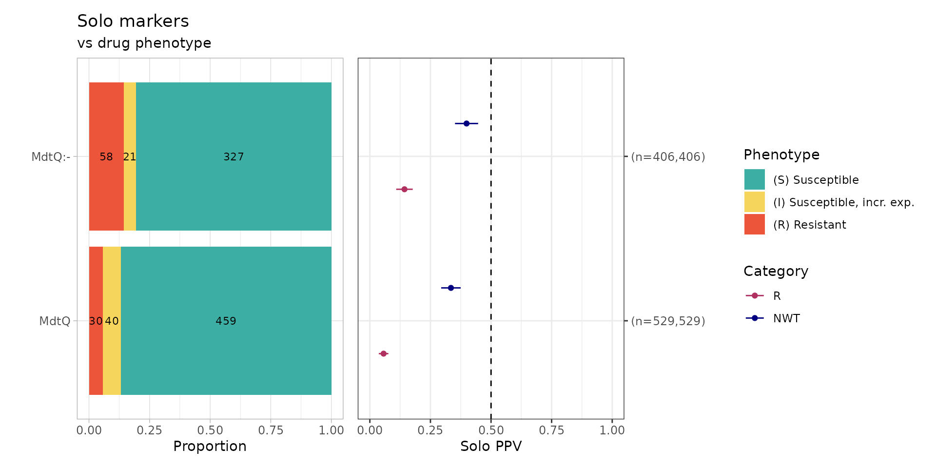
# Count number of genomes that have either `MdtQ` or `MdtQ:-`
sum(rgi_binary_matrix_prev80$MdtQ == "1" | rgi_binary_matrix_prev80$`MdtQ..-` == "1", na.rm = TRUE)
#> [1] 1429
Only MdtQ and MdtQ variants (MdtQ:-) were identified in the absence of other carbapenem resistance determinants. MdtQ is an outer-membrane porin identified in K. pneumoniae - however the primary paper by Fan, et al. only reports a clinical strain with MdtQ resistant to carbapenems, but does not show antibiotic susceptibility tests for proper controls of the same strain with MdtQ vs. without MdtQ. In addition, 96% (n=1429/1490) of the EuSCAPE K. pneumoniae genomes have MdtQ or a variant of MdtQ, therefore it could be considered a core gene. In summary, because is no compelling evidence that MdtQ confers resistance to carbapenems and that it is likely a core gene, we will exclude it from further analyses.
# Exclude MdtQ and MdtQ:- from the binary matrix
rgi_binary_matrix_prev80 <- rgi_binary_matrix_prev80 %>% select(-MdtQ, -`MdtQ..-`)
Try running the solo_ppv() function… again.
soloPPV_rgi_mero <- solo_ppv(binary_matrix = rgi_binary_matrix_prev80)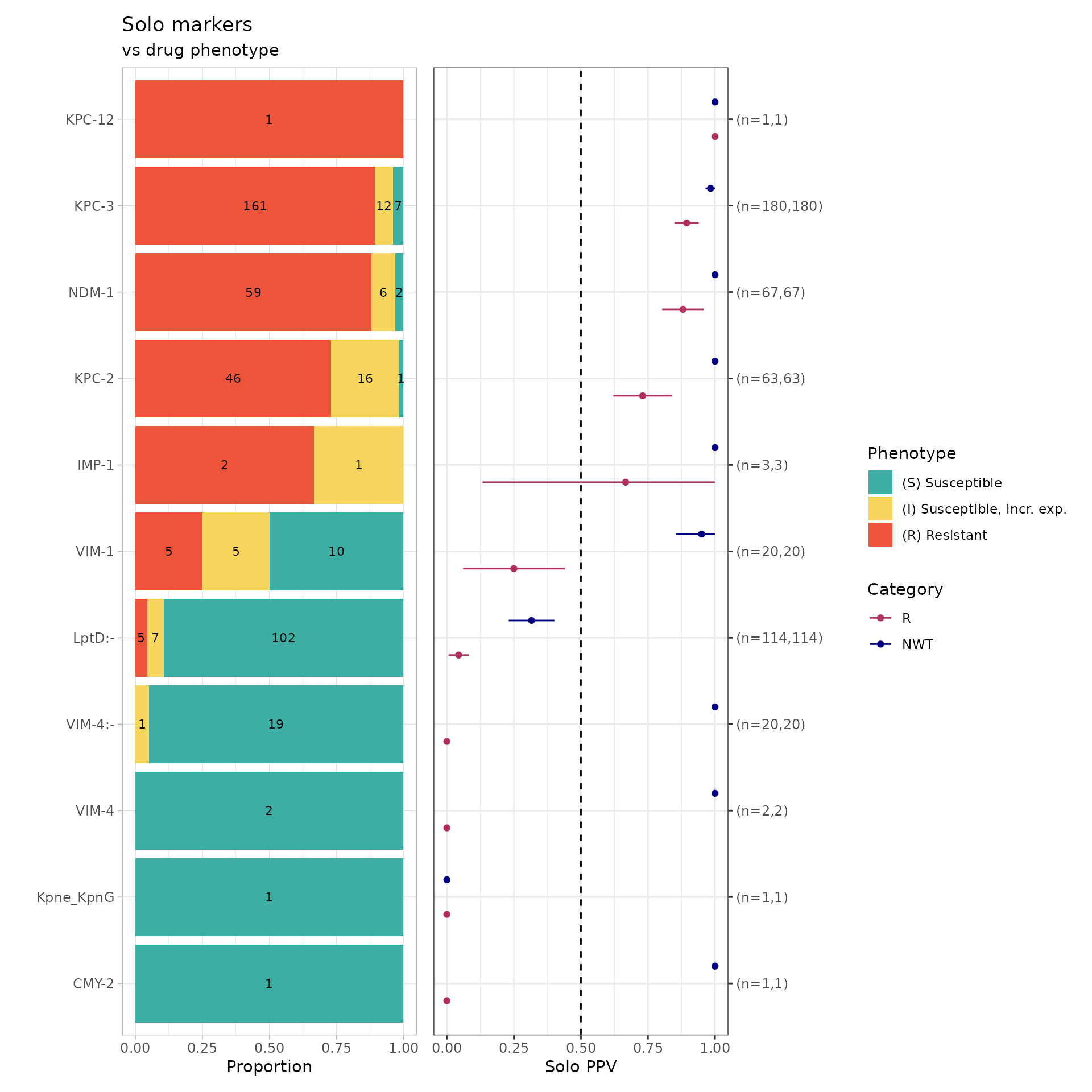
We can finally see carbapenem resistance determinants alone! Since
RGI does not detect porin defects, many AMR markers are found alone
compared to Kleborate’s and AMRFinderPlus’ solo_ppv() (see
below). For example, NDM-1 alone was found in 59 resistant genomes
(using RGI), 31 resistant genomes (using Kleborate), and 41 resistant
genomes (using AMRFinderPlus).
soloPPV_kleborate_mero
#> $solo_stats
#> # A tibble: 28 × 8
#>    marker                category     x     n    ppv     se ci.lower ci.upper
#>    <chr>                 <chr>    <dbl> <int>  <dbl>  <dbl>    <dbl>    <dbl>
#>  1 OXA-162               R            0     2 0      0        0        0
#>  2 OXA-204               R            0     1 0      0        0        0
#>  3 OmpK36:c.25C>T        R            0     6 0      0        0        0
#>  4 OmpK36:p.134_135insGD R            0     9 0      0        0        0
#>  5 VIM-1                 R            0    13 0      0        0        0
#>  6 VIM-4                 R            0     4 0      0        0        0
#>  7 OmpK36:-              R            1    71 0.0141 0.0140   0        0.0415
#>  8 OmpK35:-              R            2    49 0.0408 0.0283   0        0.0962
#>  9 OXA-48                R            6    99 0.0606 0.0240   0.0136   0.108
#> 10 KPC-3                 R            3    10 0.3    0.145    0.0160   0.584
#> # ℹ 18 more rows
#>
#> $combined_plot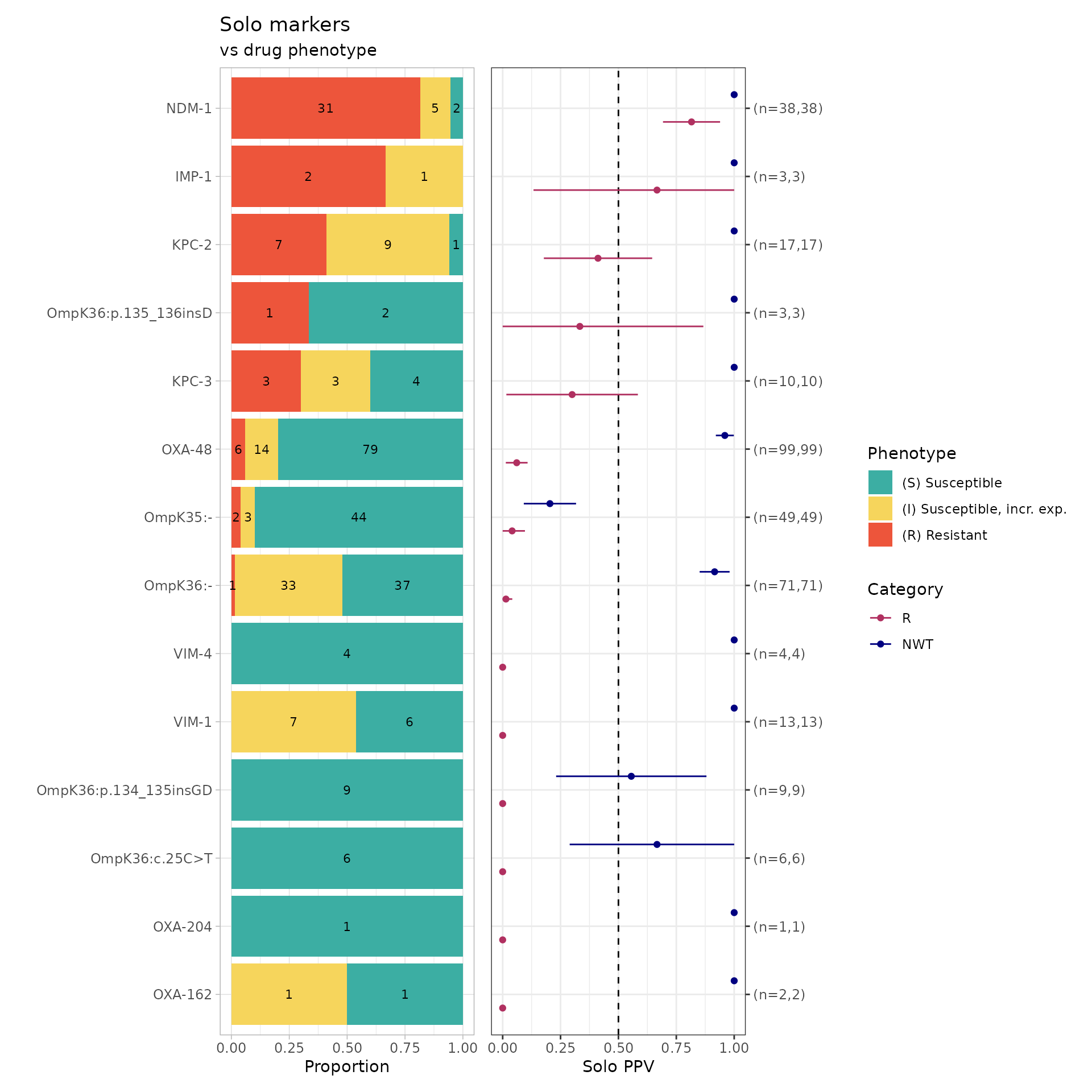
#>
#> $solo_binary
#> # A tibble: 325 × 8
#>    id           pheno ecoff    mic     R   NWT marker   value
#>    <chr>        <sir> <sir>  <mic> <dbl> <dbl> <chr>    <dbl>
#>  1 SAMEA3498967   I    NWT    4.00     0     1 OmpK36:-     1
#>  2 SAMEA3498970   I    NWT    4.00     0     1 OmpK36:-     1
#>  3 SAMEA3498975   S    NWT    2.00     0     1 OmpK36:-     1
#>  4 SAMEA3498992   S    NWT    0.50     0     1 OmpK36:-     1
#>  5 SAMEA3498996   S     WT  <=0.06     0     0 OmpK35:-     1
#>  6 SAMEA3498997   S    NWT    0.50     0     1 OmpK36:-     1
#>  7 SAMEA3498998   S    NWT    2.00     0     1 OmpK36:-     1
#>  8 SAMEA3499003   R    NWT  >32.00     1     1 NDM-1        1
#>  9 SAMEA3499004   R    NWT   32.00     1     1 OmpK36:-     1
#> 10 SAMEA3499010   S     WT  <=0.06     0     0 OmpK35:-     1
#> # ℹ 315 more rows
#>
#> $solo_binary_norange
#> NULL
#>
#> $amr_binary
#> # A tibble: 1,490 × 24
#>    id    pheno ecoff    mic     R   NWT `OmpK36..-` `OmpK35..-` `NDM-1` `OXA-48`
#>    <chr> <sir> <sir>  <mic> <dbl> <dbl>       <dbl>       <dbl>   <dbl>    <dbl>
#>  1 SAME…   I    NWT    4.00     0     1           1           0       0        0
#>  2 SAME…   S     WT  <=0.06     0     0           0           0       0        0
#>  3 SAME…   S    NWT    1.00     0     1           1           1       0        0
#>  4 SAME…   I    NWT    4.00     0     1           1           0       0        0
#>  5 SAME…   I    NWT    4.00     0     1           1           1       0        0
#>  6 SAME…   S     WT  <=0.06     0     0           0           0       0        0
#>  7 SAME…   S     WT  <=0.06     0     0           0           0       0        0
#>  8 SAME…   S    NWT    2.00     0     1           1           0       0        0
#>  9 SAME…   S     WT  <=0.06     0     0           0           0       0        0
#> 10 SAME…   S    NWT    0.50     0     1           1           0       0        0
#> # ℹ 1,480 more rows
#> # ℹ 14 more variables: `OmpK36..c.25C>T` <dbl>, `KPC-3` <dbl>,
#> #   OmpK36..p.134_135insGD <dbl>, `KPC-2` <dbl>, OmpK36..p.135_136insD <dbl>,
#> #   `OXA-204` <dbl>, `VIM-1` <dbl>, OmpK36..p.136_137insTD <dbl>,
#> #   `VIM-4` <dbl>, `KPC-12` <dbl>, `OXA-232` <dbl>, `CTX-M-33` <dbl>,
#> #   `OXA-162` <dbl>, `IMP-1` <dbl>
#>
#> $plot_order
#>               OXA-162               OXA-204        OmpK36:c.25C>T
#>             "(n=2,2)"             "(n=1,1)"             "(n=6,6)"
#> OmpK36:p.134_135insGD                 VIM-1                 VIM-4
#>             "(n=9,9)"           "(n=13,13)"             "(n=4,4)"
#>              OmpK36:-              OmpK35:-                OXA-48
#>           "(n=71,71)"           "(n=49,49)"           "(n=99,99)"
#>                 KPC-3  OmpK36:p.135_136insD                 KPC-2
#>           "(n=10,10)"             "(n=3,3)"           "(n=17,17)"
#>                 IMP-1                 NDM-1
#>             "(n=3,3)"           "(n=38,38)"
# Generate binary matrix for AMRFinderPlus
amrfp_binary_matrix <- get_binary_matrix(
  geno_table = kp_mero_amrfp,
  pheno_table = kp_mero_euscape,
  pheno_drug = "Meropenem",
  geno_class = c("Carbapenems"),
  sir_col = "pheno_eucast",
  keep_assay_values = TRUE,
  keep_assay_values_from = "mic"
)
#>  Defining NWT in binary matrix using ecoff column provided: ecoff
# Solo PPV analysis
soloPPV_amrfp_mero <- solo_ppv(binary_matrix = amrfp_binary_matrix)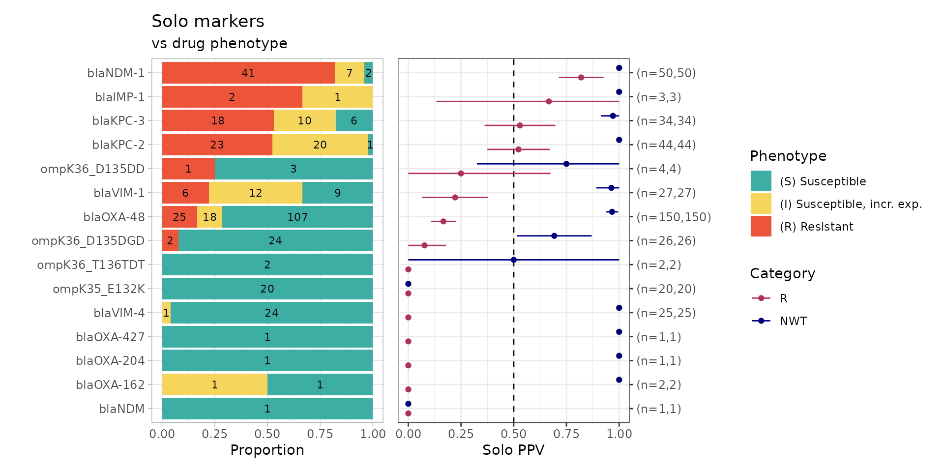
Combinatorial PPV Analysis for RGI AMR Markers
comboPPV_rgi_mero <- amr_ppv(
  binary_matrix = rgi_binary_matrix_prev80,
  order = "value",
  min_set_size = 2,
  pheno_drug = "Meropenem",
  upset_grid = TRUE,
  plot_assay = TRUE,
  assay = "mic"
)
#> Ordering markers by frequency
#> Scale for y is already present.
#> Adding another scale for y, which will replace the existing scale.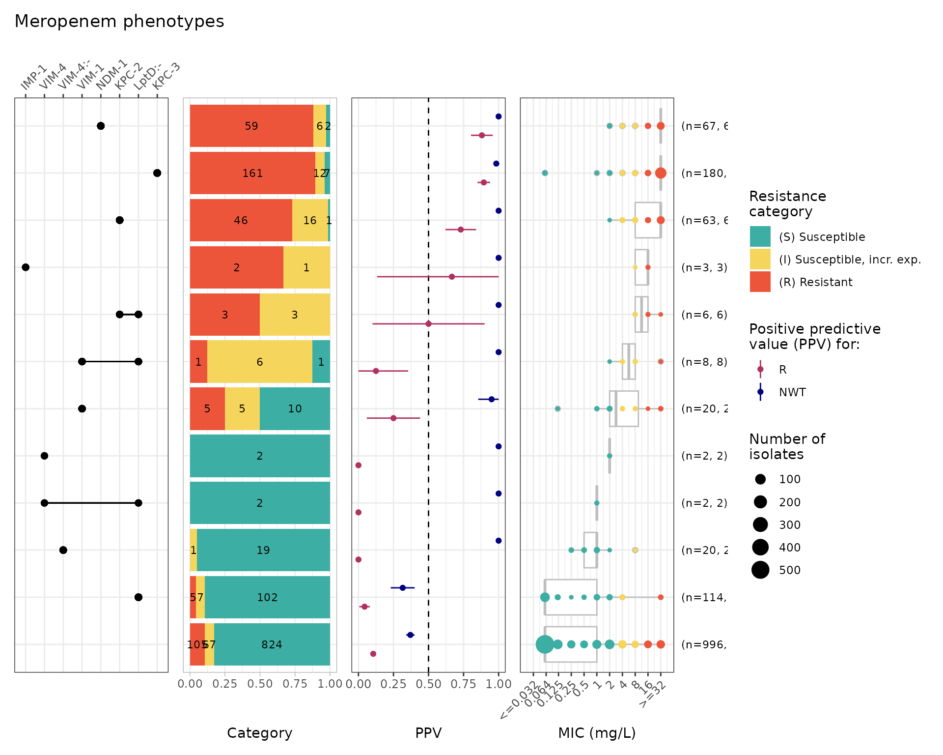
# Summary of combinatorial PPV
comboPPV_rgi_mero$summary
#> # A tibble: 21 × 21
#>    marker_list        marker_count     n combination_id    R.n  R.ppv R.ci_lower
#>    <chr>                     <dbl> <int> <fct>           <dbl>  <dbl>      <dbl>
#>  1 ""                            0   996 0_0_0_0_0_0_0_…   105 0.105     0.0863
#>  2 "IMP-1"                       1     3 0_0_0_0_0_0_0_…     2 0.667     0.133
#>  3 "CMY-2"                       1     1 0_0_0_0_0_0_0_…     0 0         0
#>  4 "KPC-12"                      1     1 0_0_0_0_0_0_0_…     1 1         1
#>  5 "Kpne_KpnG"                   1     1 0_0_0_0_0_0_0_…     0 0         0
#>  6 "VIM-4"                       1     2 0_0_0_0_0_0_1_…     0 0         0
#>  7 "VIM-4:-"                     1    20 0_0_0_0_0_1_0_…     0 0         0
#>  8 "VIM-1"                       1    20 0_0_0_0_1_0_0_…     5 0.25      0.0602
#>  9 "LptD:-"                      1   114 0_0_0_1_0_0_0_…     5 0.0439    0.00627
#> 10 "LptD:-, NDM-69:-"            2     1 0_0_0_1_0_0_0_…     0 0         0
#> # ℹ 11 more rows
#> # ℹ 14 more variables: R.ci_upper <dbl>, R.denom <int>, NWT.n <dbl>,
#> #   NWT.ppv <dbl>, NWT.ci_lower <dbl>, NWT.ci_upper <dbl>, NWT.denom <int>,
#> #   median_excludeRangeValues <dbl>, q25_excludeRangeValues <dbl>,
#> #   q75_excludeRangeValues <dbl>, n_excludeRangeValues <int>,
#> #   median_ignoreRanges <dbl>, q25_ignoreRanges <dbl>, q75_ignoreRanges <dbl>
Evidently, RGI does not detect OmpK35 or OmpK36 defects so we can only compare the carbapenemases that are detected by RGI vs. Kleborate development branch.
Compare RGI to Kleborate Genotype Results
rgi_simplified <- rgi %>%
  filter(drug_class == "Carbapenems") %>%
  filter(`Resistance Mechanism` == "antibiotic inactivation") %>%
  select(id, marker.label) %>%
  distinct() %>%
  rename(rgi = marker.label) %>%
  group_by(id) %>%
  summarise(
    rgi_markers = rgi %>%
      sort() %>%
      str_c(collapse = ";")
  )

kleborate_simplified <- kleborate_dev %>%
  filter(Kleborate_Class == "Omp_mutations" | Kleborate_Class == "Bla_Carb_acquired") %>%
  select(id, marker.label) %>%
  rename(kleborate = marker.label) %>%
  filter(!grepl("OmpK35|OmpK36", kleborate)) %>%
  group_by(id) %>%
  summarise(
    Kleborate_markers = kleborate %>%
      sort() %>%
      str_c(collapse = ";")
  )

compare_rgi_kleborate <- full_join(
  rgi_simplified,
  kleborate_simplified
)
#> Joining with `by = join_by(id)`

compare_rgi_kleborate <- compare_rgi_kleborate %>%
  rowwise() %>%
  mutate(
    Kleborate_missing = {
      rgi_vec <- str_split(rgi_markers, ";")[[1]]
      kleb_vec <- str_split(Kleborate_markers, ";")[[1]]
      missing <- setdiff(rgi_vec, kleb_vec)
      if (length(missing) == 0) NA_character_ else str_c(missing, collapse = ";")
    },
    rgi_missing = {
      rgi_vec <- str_split(rgi_markers, ";")[[1]]
      kleb_vec <- str_split(Kleborate_markers, ";")[[1]]
      missing <- setdiff(kleb_vec, rgi_vec)
      if (length(missing) == 0) NA_character_ else str_c(missing, collapse = ";")
    }
  ) %>%
  ungroup()

compare_rgi_kleborate %>% count(Kleborate_missing, sort = TRUE)
#> # A tibble: 4 × 2
#>   Kleborate_missing     n
#>   <chr>             <int>
#> 1 NA                  576
#> 2 VIM-4:-              20
#> 3 CMY-2                 1
#> 4 NDM-69:-              1
compare_rgi_kleborate %>% count(rgi_missing, sort = TRUE)
#> # A tibble: 10 × 2
#>    rgi_missing      n
#>    <chr>        <int>
#>  1 NA             371
#>  2 OXA-48         207
#>  3 KPC-3            6
#>  4 KPC-2            4
#>  5 OXA-232          4
#>  6 OXA-162          2
#>  7 CTX-M-33         1
#>  8 NDM-1            1
#>  9 NDM-1;OXA-48     1
#> 10 OXA-204          1
Combining Kleborate, AMRFinderPlus and RGI results
To merge Kleborate (development branch), AMRFinderPlus (from EBI),
and RGI results, we will combine the binary matrices generated by
get_binary_matrix().
Note that you will have to inspect how each of the AMR markers are
named and change them so that they match and can be merged, for example
AMRFinderPlus appends “bla” in front of all beta-lactamases, whereas RGI
and Kleborate do not. This assumes that the same name is
referring to the same reference sequence that is used in each
tool/database which is not necessarily true (even if we wish it
were true). Hypothetical example, the NDM-1 sequence in CARD/RGI is
ABCD vs. AMRFinderPlus NDM-1 sequence is ACCD
vs. Kleborate NDM-1 sequence is ACDD. All AMR databases
strive to use the same reference accessions and sequences, but sometimes
there can be discrepancies, which need to be kept in mind.
In the following code, unique AMR markers (i.e., only identified by
one AMR genotyper) will be have a suffix to describe the AMR genotyper
that it is found by (e.g., Kpne_KpnG will be Kpne_KpnG_rgi). AMR markers
identified by more than one genotyper will be merged, where if it was
identified by any genotyper in that sample, the binary matrix will have
a 1 (present), otherwise 0 (absent).
# Phenotype columns to remove (that we can put back in later)
cols_to_remove <- c("pheno", "ecoff", "mic", "R", "NWT")

# Remove columns
# We will be using the RGI binary matrix where core/intrinsic genes are removed
df_rgi <- rgi_binary_matrix_prev80 %>% select(-cols_to_remove)
#> Warning: Using an external vector in selections was deprecated in tidyselect 1.1.0.
#> ℹ Please use `all_of()` or `any_of()` instead.
#>   # Was:
#>   data %>% select(cols_to_remove)
#>
#>   # Now:
#>   data %>% select(all_of(cols_to_remove))
#>
#> See <https://tidyselect.r-lib.org/reference/faq-external-vector.html>.
#> This warning is displayed once per session.
#> Call `lifecycle::last_lifecycle_warnings()` to see where this warning was
#> generated.
df_kleborate <- kleborate_binary_matrix %>% select(-cols_to_remove)

# Massage AMRFinderPlus marker names to match RGI/Kleborate
df_amrfp <- amrfp_binary_matrix %>%
  select(-cols_to_remove) %>%
  rename("OmpK36..p.134_135insGD" = "ompK36_D135DGD") %>%
  rename("OmpK36..p.135_136insD" = "ompK36_D135DD") %>%
  rename("OmpK36..p.136_137insTD" = "ompK36_T136TDT")
colnames(df_amrfp) <- gsub("bla", "", colnames(df_amrfp))

# Sort each dataframe by id to make sure the samples are all in the same order
df_rgi <- df_rgi[order(df_rgi[[1]]), ]
df_amrfp <- df_amrfp[order(df_amrfp[[1]]), ]
df_kleborate <- df_kleborate[order(df_kleborate[[1]]), ]

# All column names (excluding id)
cols_rgi <- colnames(df_rgi)[-1]
cols_amrfp <- colnames(df_amrfp)[-1]
cols_kleb <- colnames(df_kleborate)[-1]

all_cols <- unique(c(cols_rgi, cols_amrfp, cols_kleb))

# Function to safely get column or return 0s
get_col <- function(df, col) {
  if (col %in% colnames(df)) {
    df[[col]]
  } else {
    rep(0, nrow(df))
  }
}

# Initialize final df (assuming same order of ids)
combined_binary_matrix <- data.frame(id = df_rgi[[1]])

# Merge all columns using OR
for (col in all_cols) {
  combined_binary_matrix[[col]] <- as.integer(
    get_col(df_rgi, col) |
      get_col(df_amrfp, col) |
      get_col(df_kleborate, col)
  )
}

# Identify unique columns (present in ONLY one binary matrix)
unique_rgi <- setdiff(cols_rgi, union(cols_amrfp, cols_kleb))
unique_amrfp <- setdiff(cols_amrfp, union(cols_rgi, cols_kleb))
unique_kleb <- setdiff(cols_kleb, union(cols_rgi, cols_amrfp))

# Rename unique columns with suffix
colnames(combined_binary_matrix)[colnames(combined_binary_matrix) %in% unique_rgi] <- paste0(unique_rgi, "_rgi")
colnames(combined_binary_matrix)[colnames(combined_binary_matrix) %in% unique_amrfp] <- paste0(unique_amrfp, "_amrfp")
colnames(combined_binary_matrix)[colnames(combined_binary_matrix) %in% unique_kleb] <- paste0(unique_kleb, "_kleborate")

# Joining back the phenotype columns
phenotype_cols <- rgi_binary_matrix_prev80 %>%
  select(id, pheno, ecoff, mic, R, NWT)

# Merge back into your final_df
combined_binary_matrix <- combined_binary_matrix %>%
  left_join(phenotype_cols, by = "id")

# Relocate phenotype columns to the front
combined_binary_matrix <- combined_binary_matrix %>%
  relocate(pheno, ecoff, mic, R, NWT, .after = id)
Solo PPV Analysis for AMRFinderPlus, RGI, Kleborate AMR Markers
combined_solo_ppv <- solo_ppv(binary_matrix = combined_binary_matrix)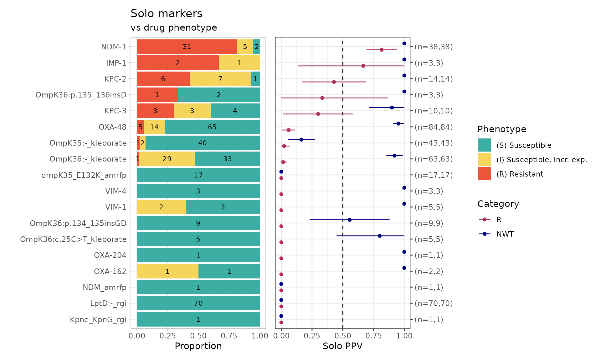 From this solo_ppv() plot, we can see that there are markers that are
found alone which have strong support for a particular phenotype, e.g.,
NDM-1 association with meropenem resistance (n=31/38 R isolates), LptD:-
identified by RGI (associated with susceptibility). Noting that LptD:-
indicates a variant of LptD, so the variants need to be further
investigated to see if there is a particular mutation/defect that is
associated with meropenem susceptibility.
From this solo_ppv() plot, we can see that there are markers that are
found alone which have strong support for a particular phenotype, e.g.,
NDM-1 association with meropenem resistance (n=31/38 R isolates), LptD:-
identified by RGI (associated with susceptibility). Noting that LptD:-
indicates a variant of LptD, so the variants need to be further
investigated to see if there is a particular mutation/defect that is
associated with meropenem susceptibility.
Another way to investigate the association between AMR markers and
meropenem susceptibility is to use the amr_logistic()
function to perform logistic regression to analyse the relationship
between the markers and a specified antibiotic.
Logistic regression for AMRFinderPlus, RGI, Kleborate AMR Markers
combined_logist <- amr_logistic(
  binary_matrix = combined_binary_matrix,
  pheno_drug = "meropenem",
  ecoff_col = "ecoff",
  maf = 10, # filter for AMR markers in at least 10 samples
  single_plot = TRUE
)
#> ...Fitting logistic regression model to R using logistf
#>    Filtered data contains 1490 samples (391 => 1, 1099 => 0) and 14 variables.
#> ...Fitting logistic regression model to NWT using logistf
#>    Filtered data contains 1490 samples (780 => 1, 710 => 0) and 14 variables.
#> Generating plots
#> Plotting 2 models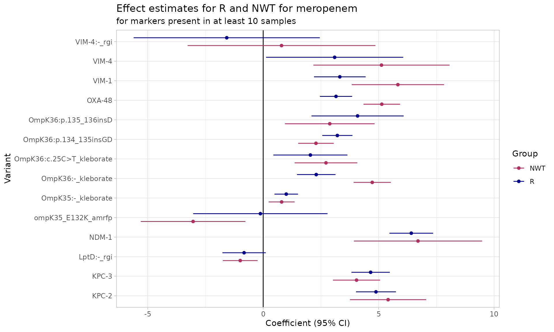
# model coefficients
combined_logist$modelR
#> # A tibble: 15 × 5
#>    marker                      est ci.lower ci.upper          pval
#>    <chr>                     <dbl>    <dbl>    <dbl>         <dbl>
#>  1 (Intercept)              -5.23    -5.91    -4.55  0
#>  2 NDM-1                     6.41     5.47     7.36  0
#>  3 KPC-3                     4.65     3.82     5.48  0
#>  4 KPC-2                     4.88     4.02     5.75  0
#>  5 LptD:-_rgi               -0.828   -1.77     0.111 0.0839
#>  6 VIM-1                     3.32     2.20     4.44  0.00000000623
#>  7 VIM-4:-_rgi              -1.58    -5.61     2.45  0.443
#>  8 VIM-4                     3.09     0.124    6.07  0.0411
#>  9 OXA-48                    3.15     2.46     3.85  0
#> 10 OmpK36:p.134_135insGD     3.21     2.56     3.87  0
#> 11 OmpK36:p.135_136insD      4.09     2.09     6.08  0.0000597
#> 12 ompK35_E132K_amrfp       -0.122   -3.03     2.79  0.935
#> 13 OmpK36:-_kleborate        2.30     1.46     3.13  0.0000000689
#> 14 OmpK35:-_kleborate        0.998    0.489    1.51  0.000123
#> 15 OmpK36:c.25C>T_kleborate  2.04     0.440    3.65  0.0125
#> Use ggplot2::autoplot() on this output to visualise
A coefficient above zero indicates that the presence of the AMR marker increases the likelihood of resistance, whereas a coefficient below zero indicates a decrease in probability of resistance. From the plot above showing AMR markers found in more than 10 isolates, majority have a positive association with resistance with the exception of LptD:- (identified by RGI), ompK35_E132K (identified by AMRFinderPlus), and VIM-4:- (identified by RGI).
Combinatorial PPV Analysis for AMRFinderPlus, RGI, Kleborate AMR Markers
comboPPV_combined_mero <- amr_ppv(
  binary_matrix = combined_binary_matrix,
  order = "value",
  min_set_size = 2,
  pheno_drug = "Meropenem",
  upset_grid = TRUE,
  plot_assay = TRUE,
  assay = "mic"
)
#> Ordering markers by frequency
#> Scale for y is already present.
#> Adding another scale for y, which will replace the existing scale.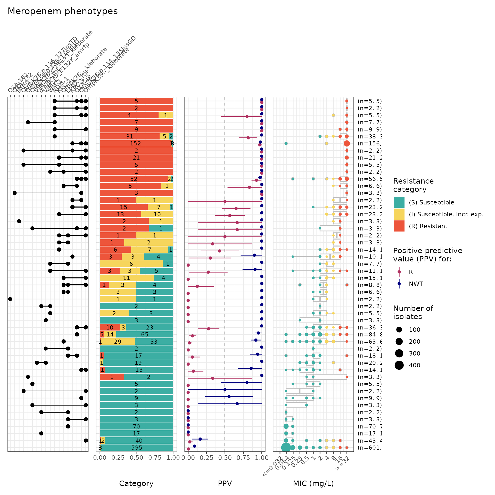
comboPPV_combined_mero$summary
#> # A tibble: 86 × 21
#>    marker_list        marker_count     n combination_id   R.n   R.ppv R.ci_lower
#>    <chr>                     <dbl> <int> <fct>          <dbl>   <dbl>      <dbl>
#>  1 ""                            0   601 0_0_0_0_0_0_0…     3 0.00499          0
#>  2 "OmpK36:c.25C>T_k…            1     5 0_0_0_0_0_0_0…     0 0                0
#>  3 "OmpK35:-_klebora…            1    43 0_0_0_0_0_0_0…     1 0.0233           0
#>  4 "OmpK35:-_klebora…            2     3 0_0_0_0_0_0_0…     0 0                0
#>  5 "OmpK36:-_klebora…            1    63 0_0_0_0_0_0_0…     1 0.0159           0
#>  6 "OmpK36:-_klebora…            2     1 0_0_0_0_0_0_0…     1 1                1
#>  7 "OmpK36:-_klebora…            2    15 0_0_0_0_0_0_0…     0 0                0
#>  8 "OXA-162"                     1     2 0_0_0_0_0_0_0…     0 0                0
#>  9 "OXA-427_amrfp, O…            2     1 0_0_0_0_0_0_0…     0 0                0
#> 10 "NDM_amrfp"                   1     1 0_0_0_0_0_0_0…     0 0                0
#> # ℹ 76 more rows
#> # ℹ 14 more variables: R.ci_upper <dbl>, R.denom <int>, NWT.n <dbl>,
#> #   NWT.ppv <dbl>, NWT.ci_lower <dbl>, NWT.ci_upper <dbl>, NWT.denom <int>,
#> #   median_excludeRangeValues <dbl>, q25_excludeRangeValues <dbl>,
#> #   q75_excludeRangeValues <dbl>, n_excludeRangeValues <int>,
#> #   median_ignoreRanges <dbl>, q25_ignoreRanges <dbl>, q75_ignoreRanges <dbl>